This article provides step-by-step instructions on trying out FreeCAD Workbench for CFD (Computational Fluid Dynamics) using OpenFOAM v2106 on a personal computer running on Ubuntu 21.04.
The instructions given are for a Ubuntu 21.04 system, but it should also work for Ubuntu 20.04 and other Ubuntu-compatible distributions with Pop!_OS inclusive.
Preparation
Base components
1: FreeCAD 0.19.x AppImage: If you don’t have FreeCAD installed, you may refer to the latest FreeCAD installation tutorial from Solvercube LearnPress (registration not required for free articles). Also check out channel videos from Solvercube Channel.
2: OpenFOAM v2106: To install OpenFOAM, refer to the latest OpenFOAM installation tutorial from Solvercube LearnPress (registration not required for free articles). Also check out channel videos from Solvercube Channel.
3: ParaView 5.9.1: To install ParaView, refer to the latest ParaView installation tutorial from Solvercube LearnPress (registration not required for free articles). Also check out channel videos from Solvercube Channel.
FreeCAD configuration (for this tutorial)
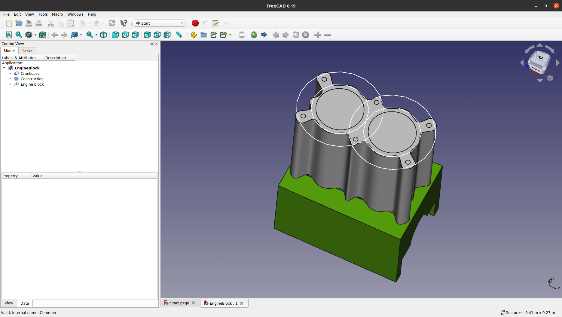
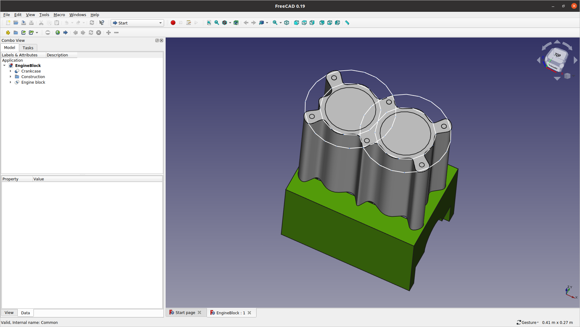
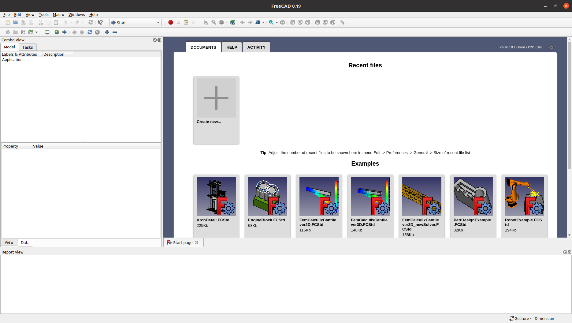
Launch FreeCAD, and open one of the example models from the Start page. Right-click on the graphics screen to select . Under this scheme, mouse operations are as follows:
-
Left button clicks on a geometrical entity: selects a single entity (e.g. a vertex, an edge, a face, etc.)
-
Left button double-click on a geometrical entity: selects the entity in the highest topological hierarchy (for example, the body containing a selected edge)
-
Left button pressed and moving around: rotates the view angle
-
Right button: opens the FreeCAD context menu
-
Right button pressed and moving around: moves the viewport laterally (i.e. panning)
-
Middle mouse click over a geometrical entity: centres the viewport around the clicked entity
-
Mouse wheel: zooms in and out the viewport, with the current cursor point being the scaling origin
You can also control the viewport using the Keyboard Navigation keys:
-
Ctrl++ and Ctrl+-: zooms in and out, respectively
-
The arrow keys, ◄ ► ▲ ▼: shifts the viewport left/right and up/down, respectively
-
Shift+◄ and Shift+►: rotates the view angle by 90 degrees around the screen’s normal axis (i.e. z-rotation)
-
The numeric keys, 0 1 2 3 4 5 6: there are seven (7) pre-defined views, that are, Isometric, Front, Top, Right, Rear, Bottom, and Left.
-
Pressing V then F: sets the viewport to fit the visible object(s)
-
Pressing V then O: sets the camera in Orthographic view
-
Pressing V then P; sets the camera in Perspective view
-
Pressing and holding Ctrl: allows you to select more than one entity (i.e. multiple selections).
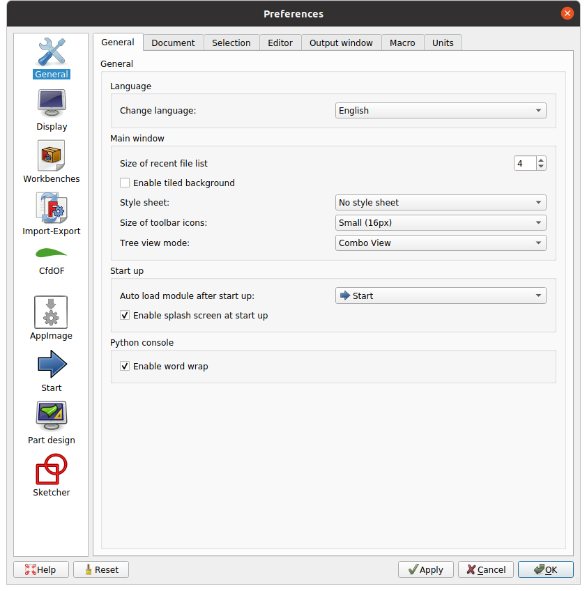
Note that FreeCAD GUI (Graphical User Interface) has many toolbar icons to boost productivity. I suggest reducing the toolbar icons size so that more icons be visible at once: Visit the menu, and select Small (16px) for the Size of toolbar icons (from the Main window section).
Also, from the main GUI layout, relocate the View toolbar
from the default position (the forefront of the second row) to the rear end of the first row. It will leave more space spared for the workbench tools we are going to use in this tutorial.
CFD Workbench Exercise
Unlike the FEM Workbench, the CFD counterpart is less standardised in FreeCAD, and you have to install your preferred extension to operate as a Workbench. In this article, we will try the CfdOF addon. Also, another addon module called Plot is required to process residuals plotting.
0: Installing Addons (required only once)
0.1: Launch FreeCAD and go to the menu. Locate the Plot addon and click the Install/update selected button to install it. When the the process is complete, shut down the Addon Manager by clicking Close, and then restart FreeCAD.
0.2: In the same manner, install the CfdOF addon and restart FreeCAD accordingly.
1: Initial configuration (for each session)
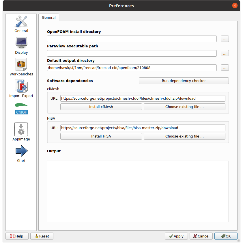
1.1: Start FreeCAD from a local work folder. Visit the Preferences panel (i.e. ) and specify the local folder for the CfdOF solution data.
-
Do not install cfMesh from this panel because OpenFOAM v2106 has this module already.
-
HiSA refers to a specialist code for the high speed aerodynamic developed and maintained by Johan Heyns et al. This is beyond the scope of the current CFD Workbench exercise.
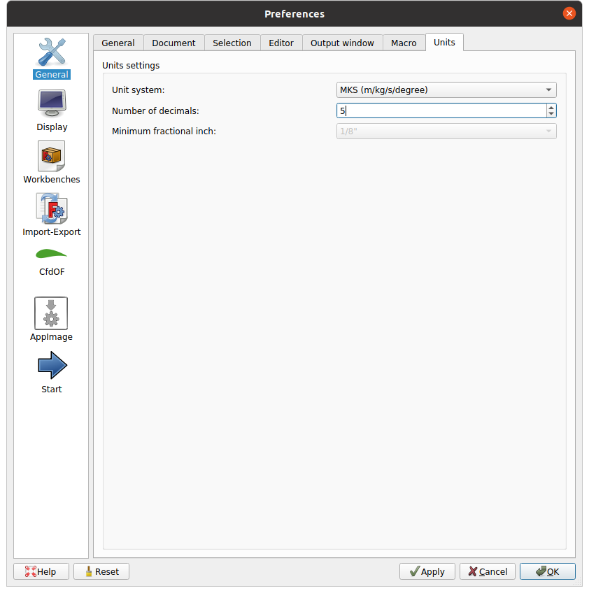
1.2: Also, I prefer to be working with the MKS (m/kg/degree) units — i.e. rather than the CAD-conventional mm-based system. Change the Number of decimals value to 5 accordingly.
2: Geometry creation
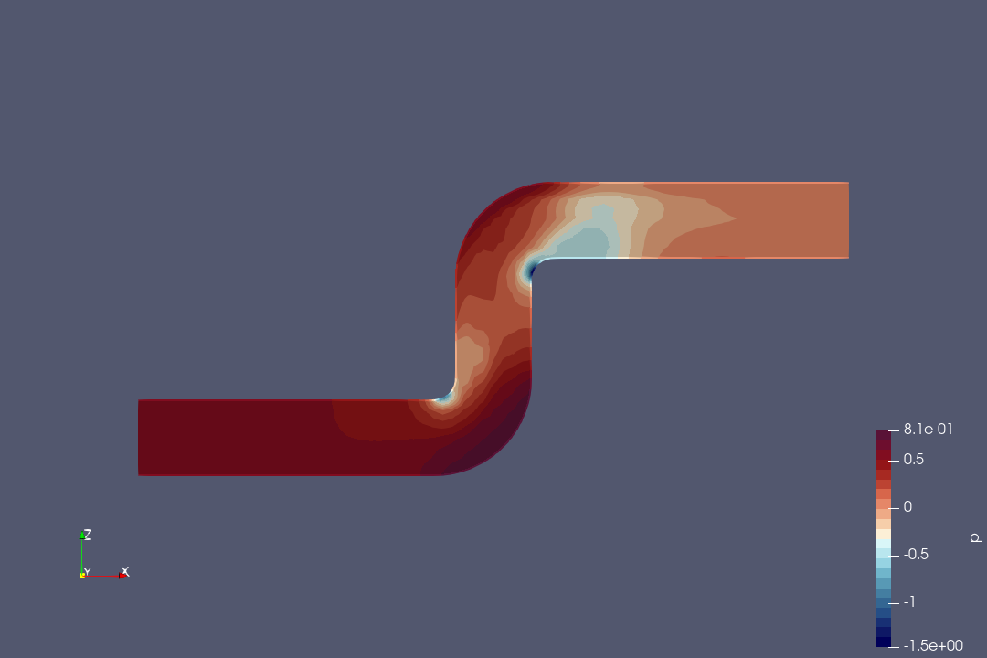
To try out the CFD Workbench, we will create an S-shaped pipe of a constant circular cross-section (16" SCH 40). We then solve the internal flow field for the water transport, with turbulence modelling inclusive.
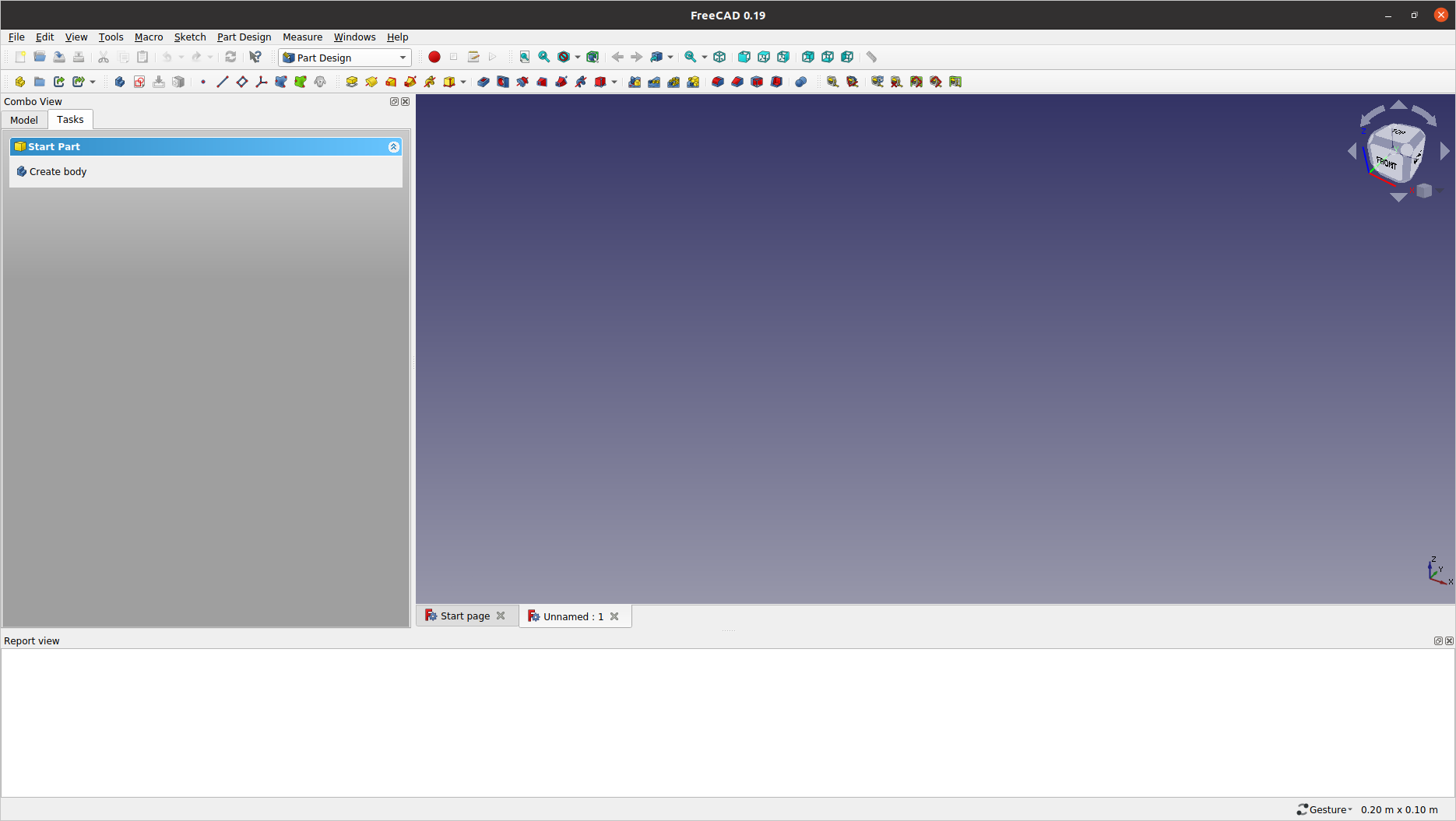
2.1: Select Part Design from the workbench selector (currently showing as ![]() ). Click the
). Click the ![]() (
(Create a new document) icon in the toolbar area to start the Part Design module.
2.2: Let us close (or detach) the Report view panel from the layout for now — either using the menu or by the panel’s close button. (It will come back anyway whenever FreeCAD needs to inform you of something.)
2.3: Click Create body under the Tasks tab in the Combo View panel; This area will be dubbed simply as the Tasks pane from now on — unless a specific task panel name is better mentioned.
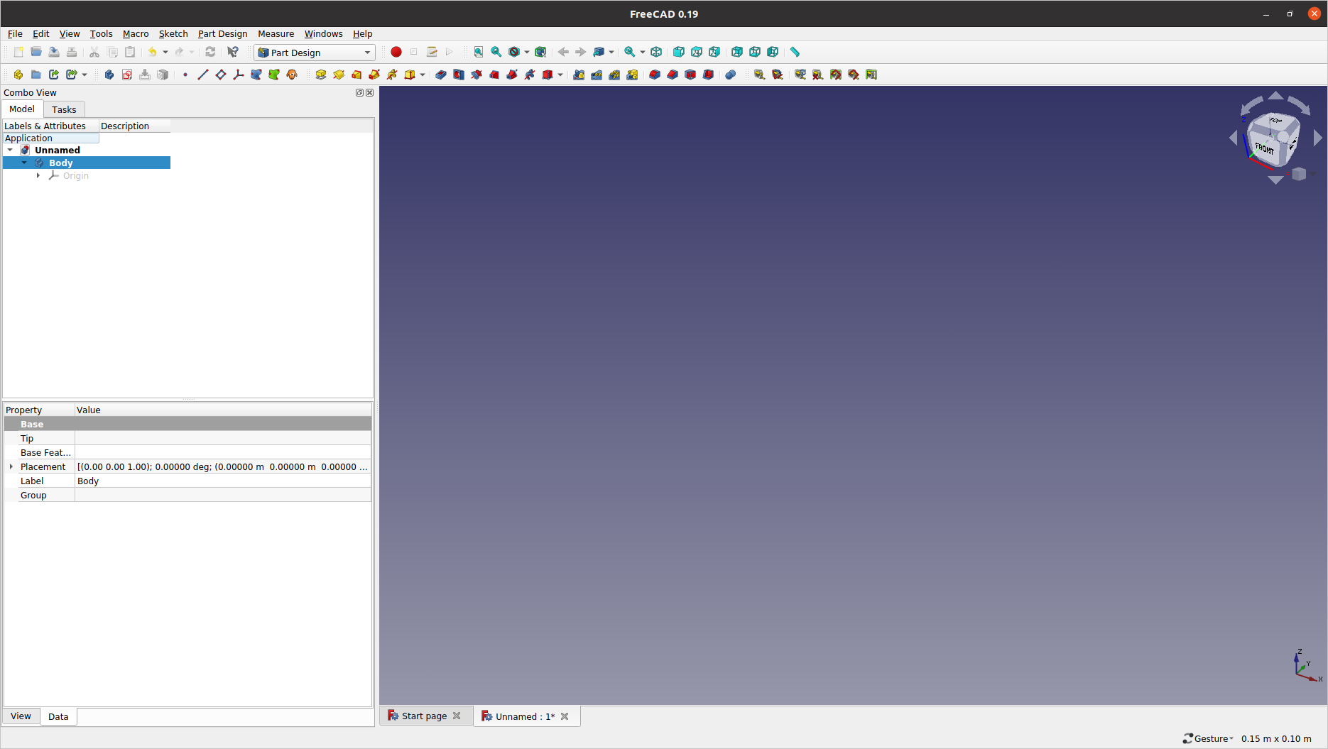
2.4: Click the Model tab to switch to the modelling tree view. See that one (and only) Body object is added under the Unnamed document root. Click the ![]() (
(Create a new sketch) icon from the toolbar to invoke the Sketcher module.
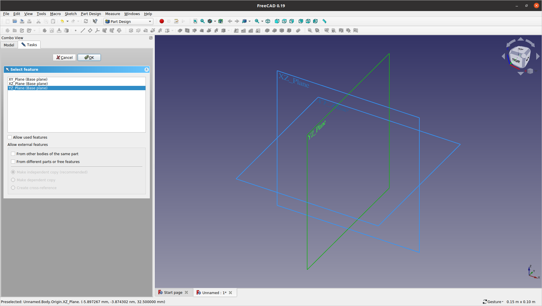
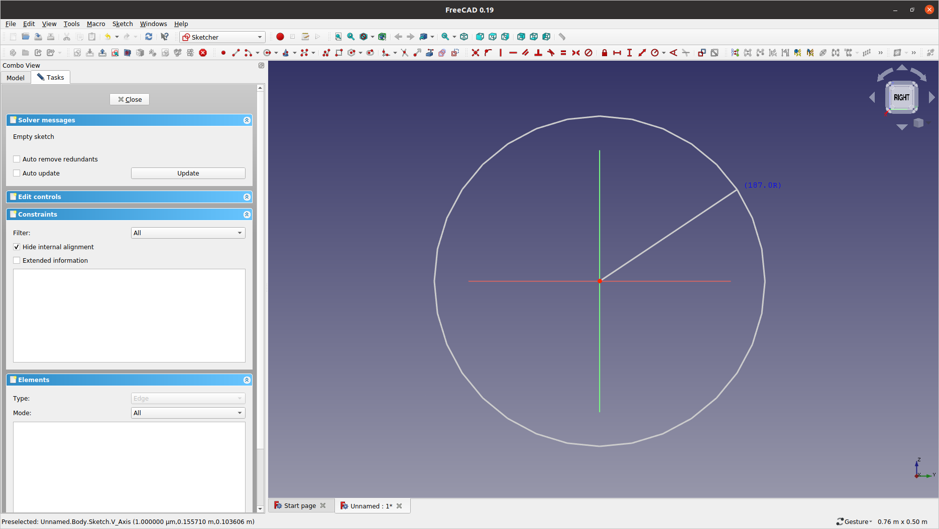
2.5: First, we will create a circle with 381 mm of (inner) diameter to define the cross-section. Select YZ_Plane either from the graphics area or the list in the Tasks pane. Click OK to confirm the plane selection.
2.6: Click ![]() (
(Create a circle in the sketch), hover the mouse cursor towards the origin point — until the point colour turns to grey — to pick it as the centre of the radius. Then, click anywhere on the +X+Y quadrant to define the 2D circular wireframe.
-
Base sketches do not have to be precise but you can make the drawing as close to the desired dimension by combining mouse wheel (zooming) and right-mouse button (panning).
-
If the output from any sketch operation is not satisfactory, you can undo it by pressing Ctrl+Z and start over.
-
You can also delete any "completed" feature from the model tree — as long as this will not deteriorate the modelling hierarchy. (If you leave the Tasks pane with any unit operation panel open, the unit operation is not complete yet.)
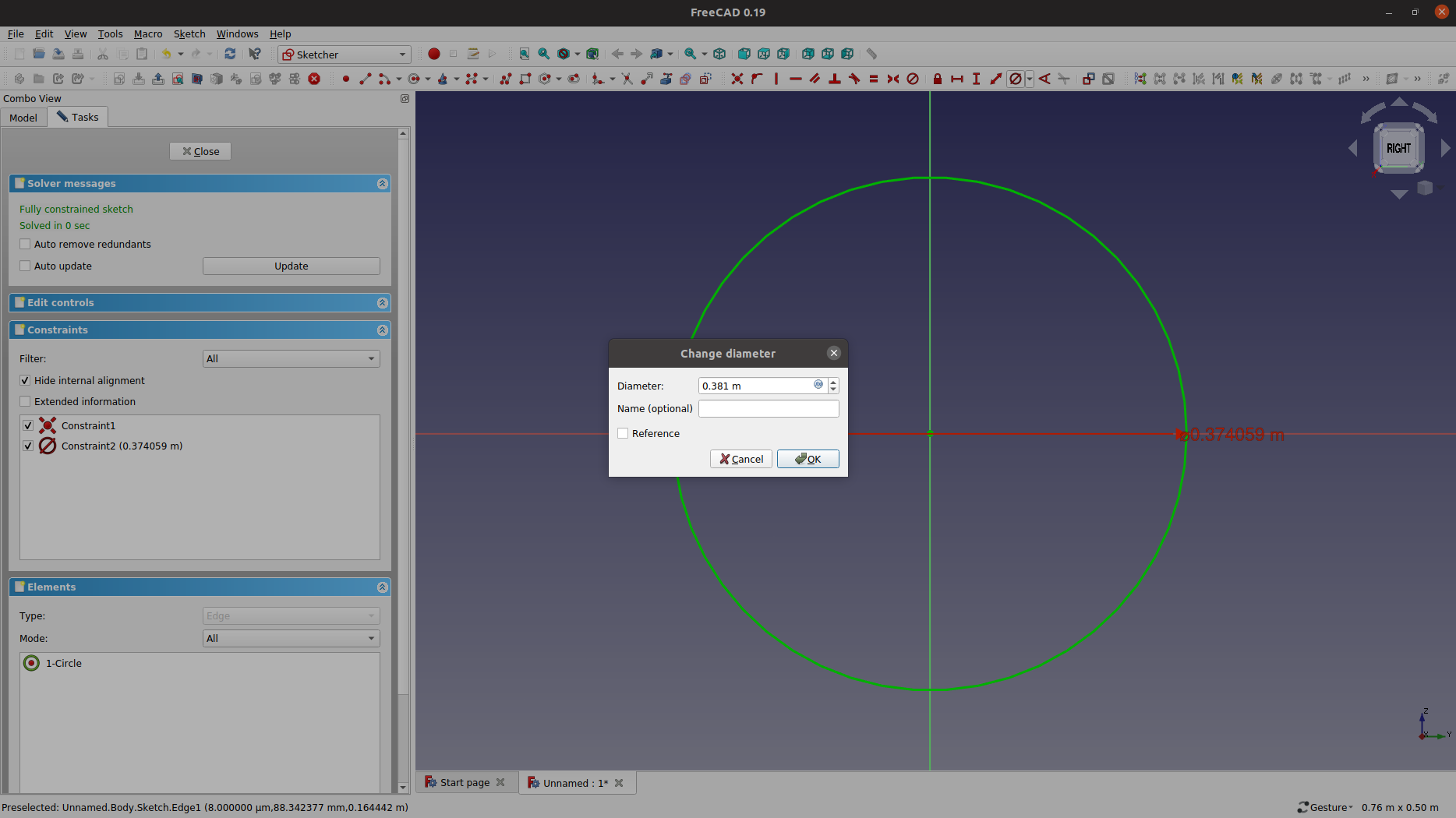
2.7: Click the ![]() (
(Constrain diameter) icon from the toolbar (You may need to click the small triangle on the right of the ![]() (
(Constrain radius) icon). Select the circumferential edge to enter 0.381 m — or 381 mm — for the Diameter in the Change diameter dialog, and then click OK. Confirm the sketch by clicking Close in the Task pane.
-
In FreeCAD, many unit operations (e.g. drawing lines, assigning dimension values, etc) are identified by the ghost graphics attached to the mouse cursor. Clicking the right mouse button anytime ends the current unit operation returning the cursor to the normal arrow.
-
If you double-click on the dimension graphic while in your selection mode (i.e. normall arrow cursor), it will bring you back to the dimension input dialog.
2.8: Make the viewport to fit to the geometry — either using the view control context menu (right click on an empty spot) or by pressing the V F key combination.

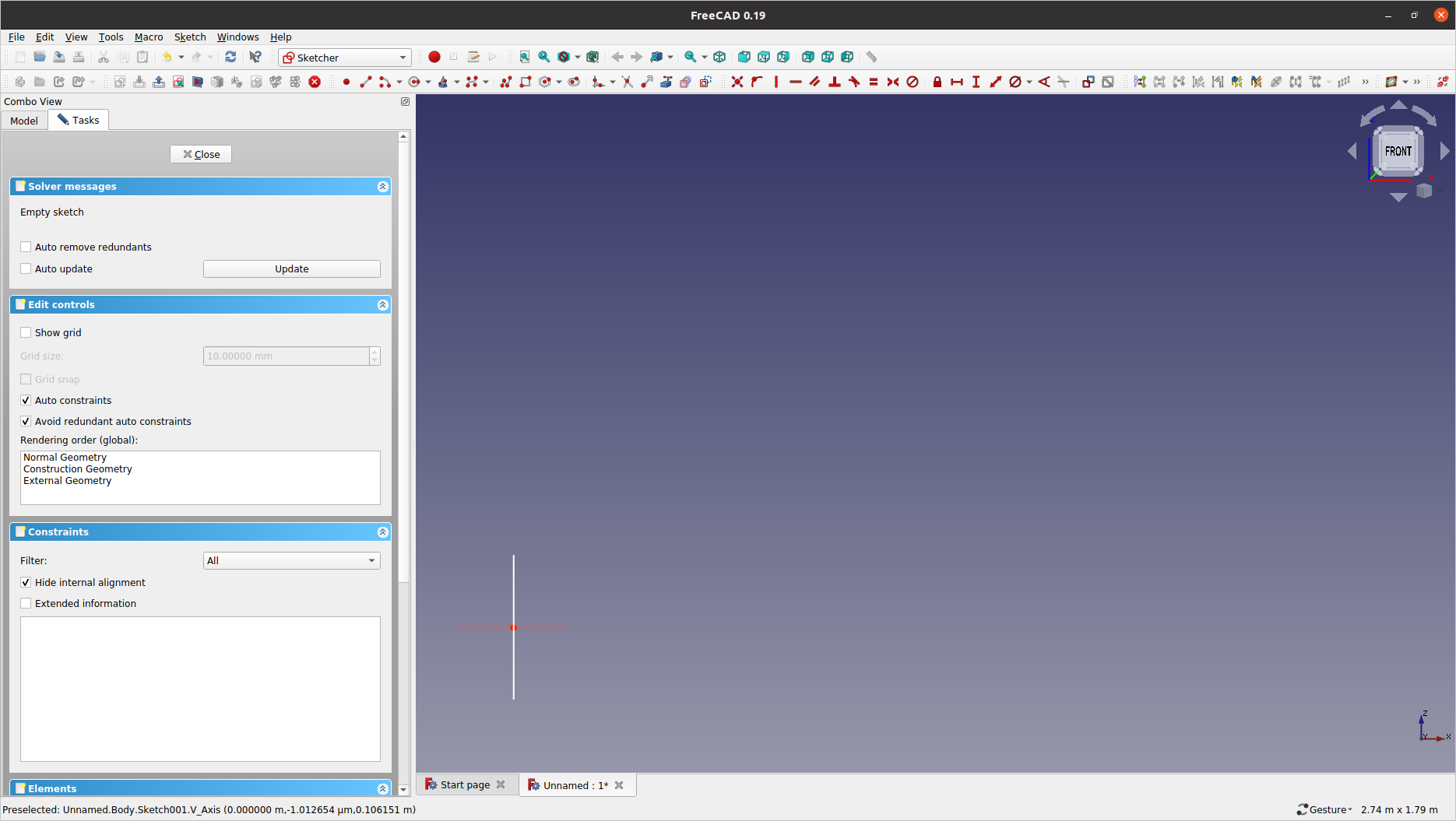
2.9: Now, we will create another wireframe to define the path profile. Click ![]() (
(Create a new sketch) again, select XZ_Plane, and then click OK. Adjust the graphics view so that the previous sketch projection (showing as a white line) be positioned in the lower-left corner.
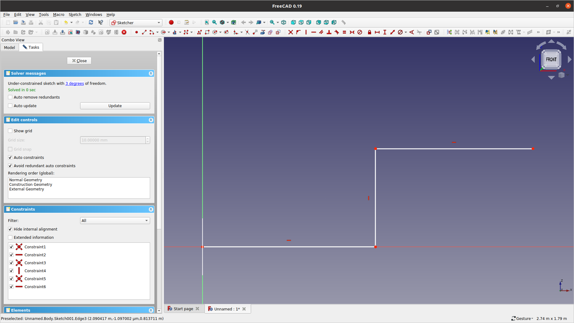
2.10: Click the ![]() (
(Create a polyline) icon from the toolbar, and starting from the origin point, draw three (3) line segments (similar to the below example). Make sure each line segment be defined with either the horizontal (![]() ) or vertical constraint (
) or vertical constraint (![]() ) imposed. Finish creating the polyline by clicking the right mouse button.
) imposed. Finish creating the polyline by clicking the right mouse button.
-
You can check whether you are imposing the coincident constraint on the start point, by the change of vertex colour and with the ghost cursor image (
 ). That said, you can always assign such constraints after the geometry creation.
2.11: We will then define two (2) 90° bends between line segments. Click ![]() (
(Create a fillet) from the toolbar, pick the first edge and then do the vertical one to insert the first fillet. You do not need to press and hold the Ctrl key as the filleting naturally expects two (2) consecutive inputs. With the ghost cursor still attached — i.e. you being in the filleting mode (if not, click ![]() again) — create the second fillet between the vertical and the last edges.
again) — create the second fillet between the vertical and the last edges.
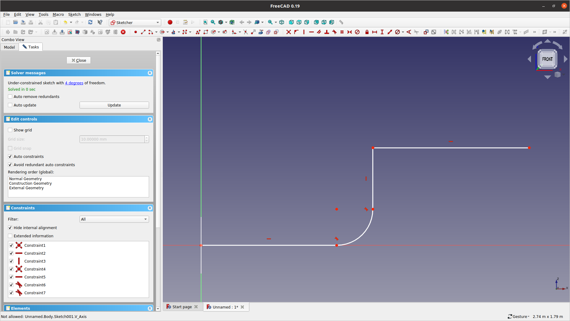
2.12: Finalise the profile sketch by assigning the following dimensional values:
-
Using
 , assign the length of
 1.5 m— or1500 mm— to the two (2) horizontal segments -
Using
 , assign the height of
 0.5 m— or500 mm— to the vertical segment -
Using
 , assign the radius of
 0.3 m— or300 mm— to the two (2) fillet sections

-
Again, to change the assigned dimensional value, check first if the mouse cursor is the normal arrow (do right-click on an empty spot if not), and then double-click the target dimension either from the graphics window or from the
Constraintslist in the Tasks pane.
2.13: When the profile sketch is complete, click Close in the Tasks pane to exit from the Sketcher. Adjust the viewport so that you can see the two (2) sketches in the graphics screen.
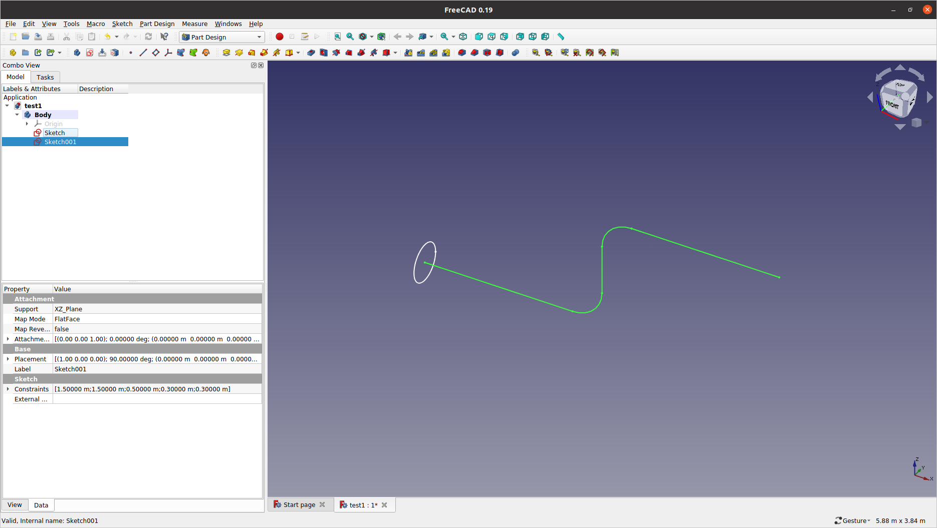
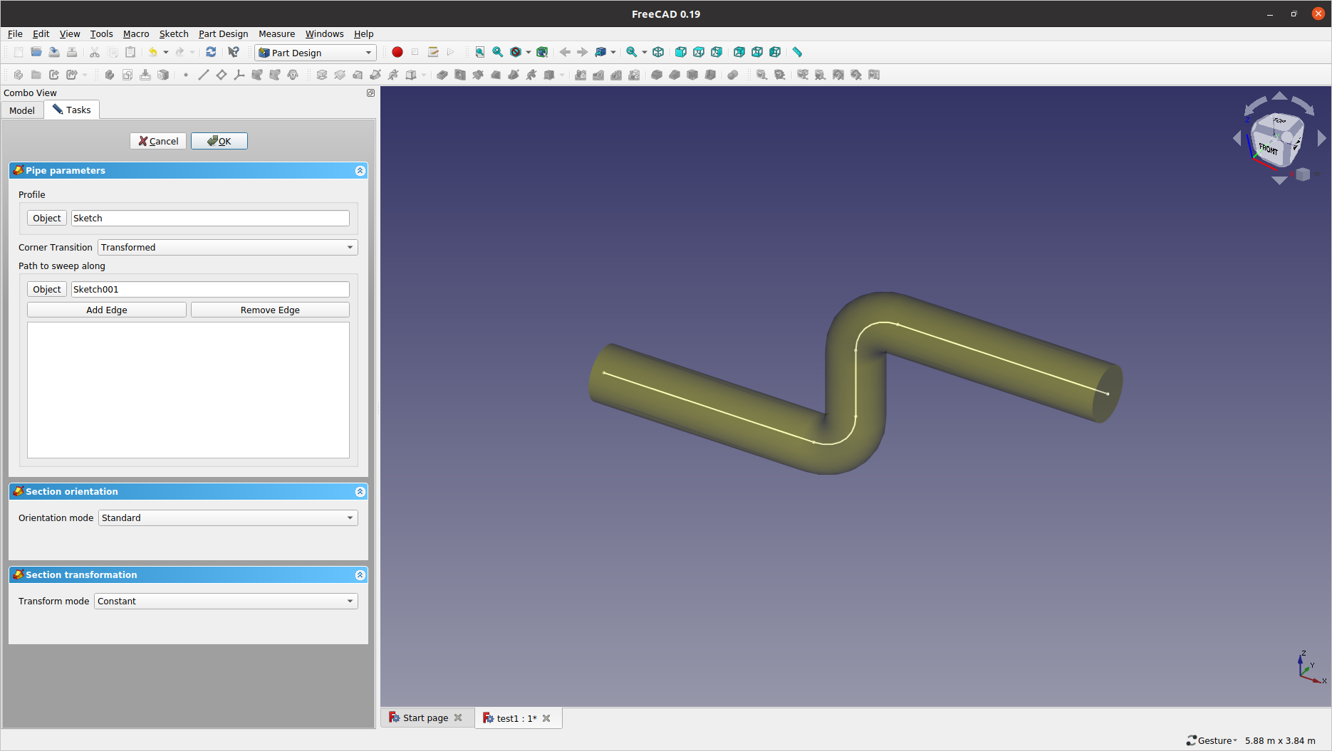
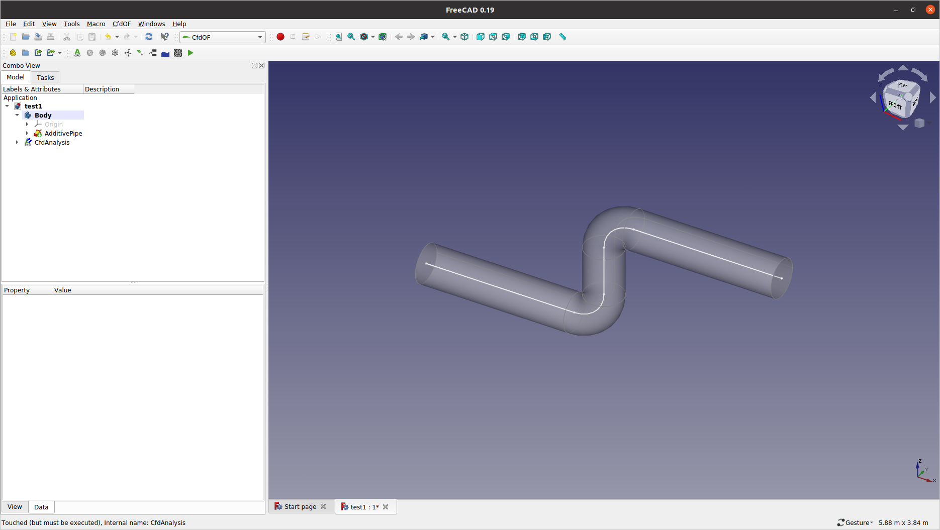
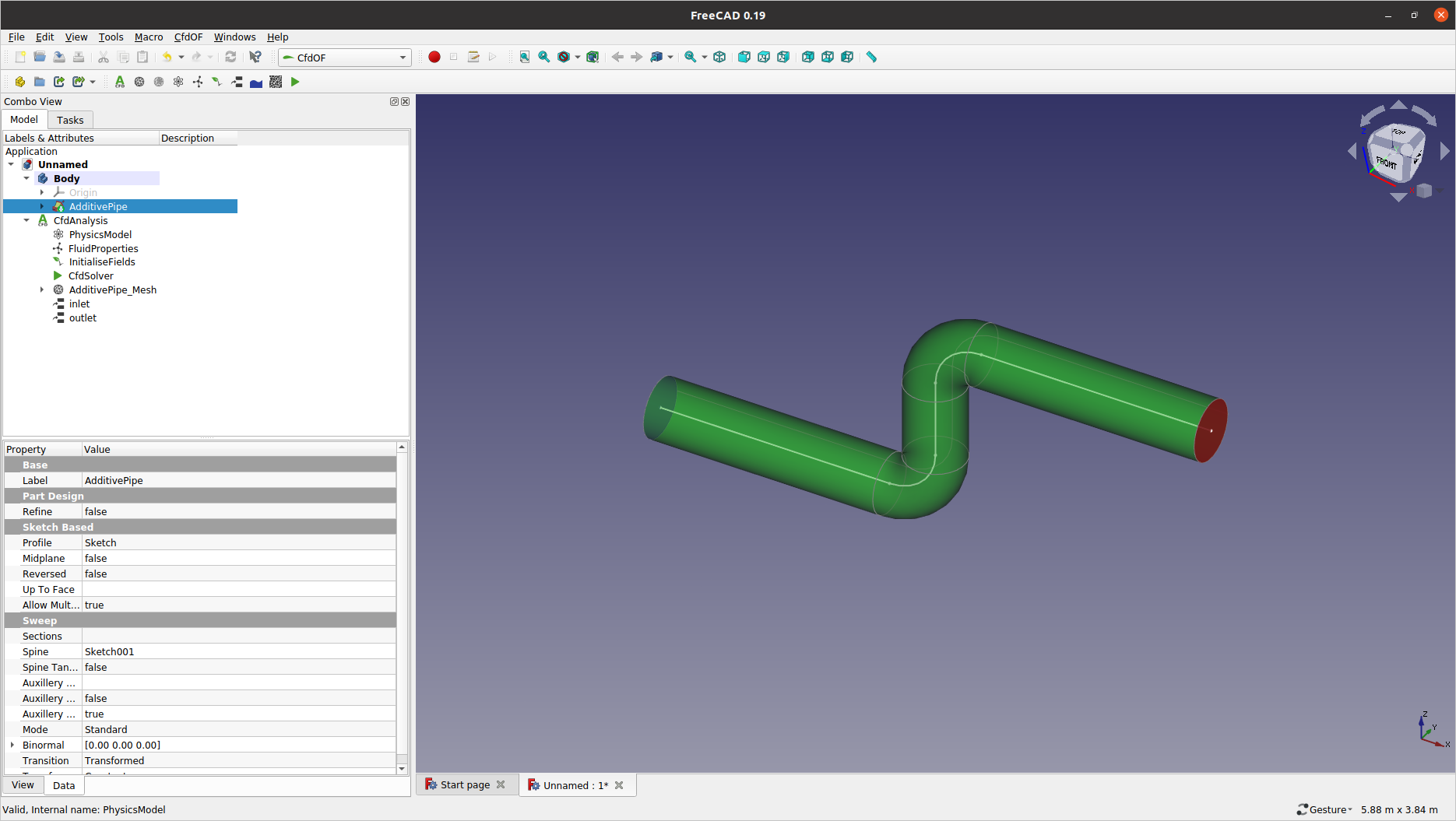
2.14: Now, with both Sketch and Sketch001 selected in the model tree, click the ![]() (
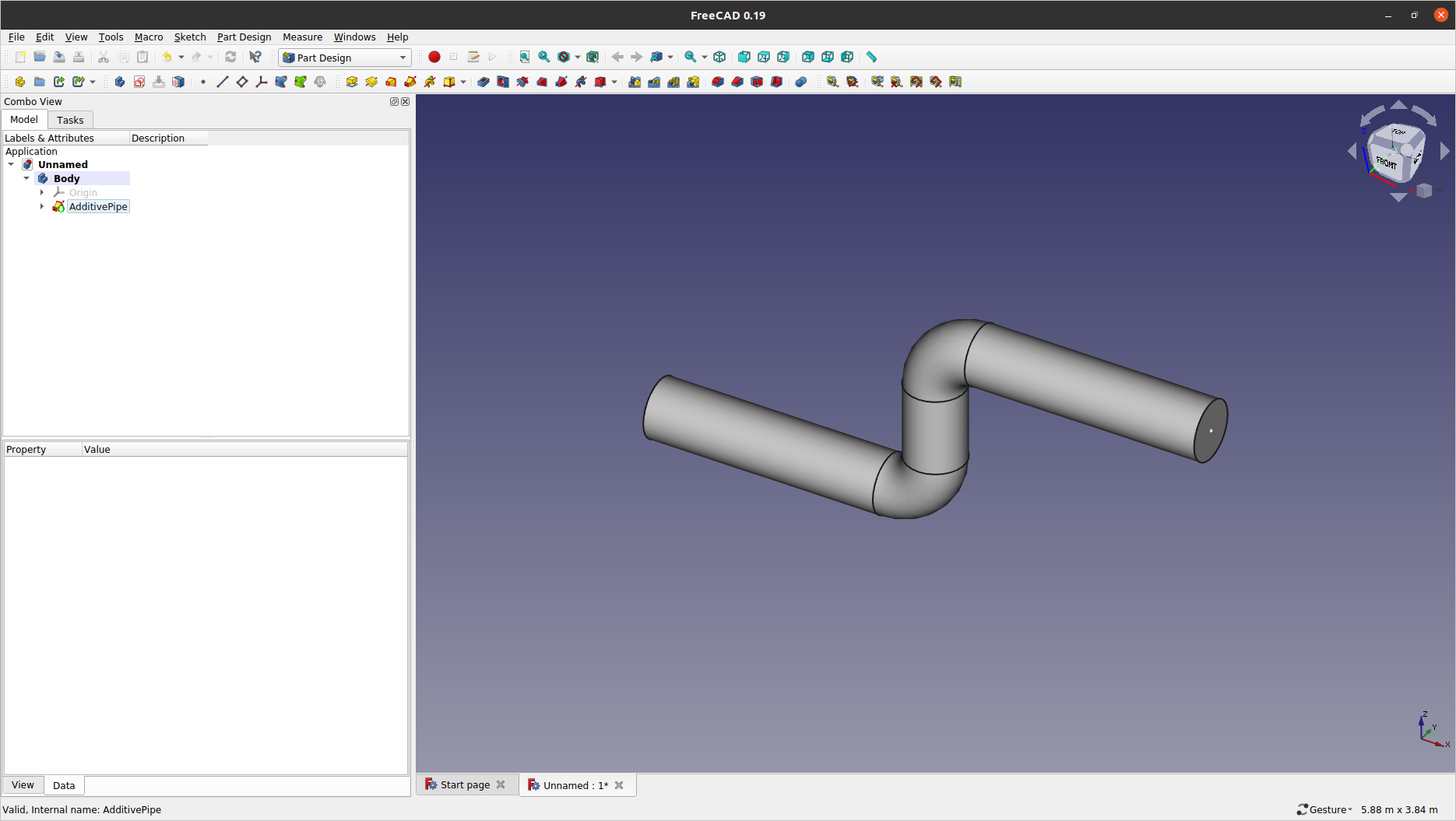
(Sweep a selected sketch) icon to build the pipe section. Click OK in the Tasks pane to confirm.
-
If in any case FreeCAD fails in discerning which object to be the profile and which one the path, remedy the assignments from the
Pipe parameterspanel.
2.15: Save the current FreeCAD document to a local work folder before we proceed with the CFD Workbench.
3: Preliminary mesh generation
Our preferred meshing tool for the CFD Workbench is the cfMesh software developed by Creative Fields Holdings Ltd. It has been incorporated since OpenFOAM v1712, thus you do not need to install it externally.
3.1: Select CfdOF from the workbench selector, and then click the ![]() (
(Create an analysis container with a CFD solver) icon from the toolbar. Make sure one (and only) CfdAnalysis object is added to the model tree.
3.2: Select the AdditivePipe object in the model tree to define the meshing scope, and then click ![]() (
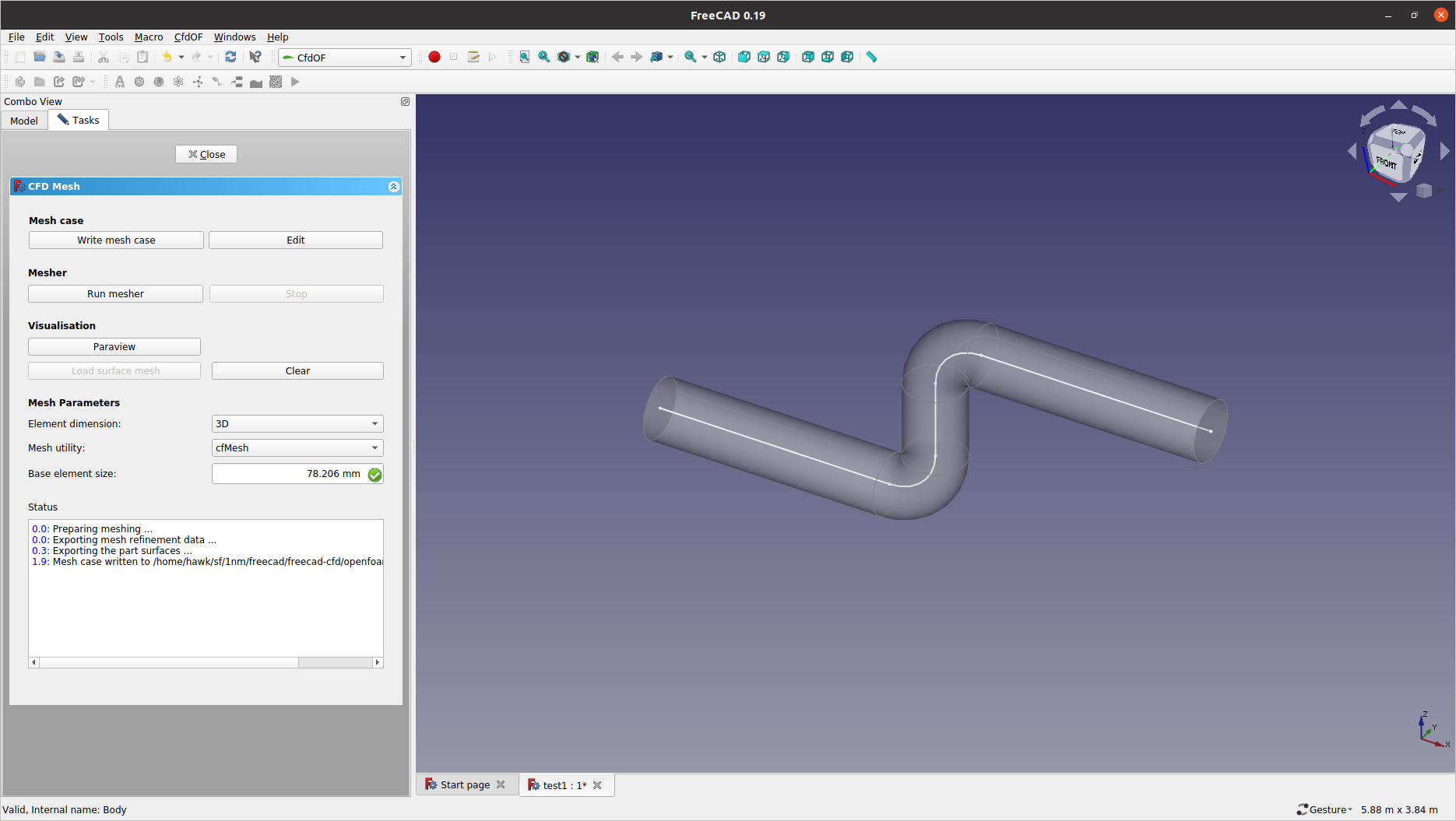
(Create a mesh) from the toolbar. When the CFD Mesh panel opens, initiate your meshing task by clicking the Write mesh case button.
-
You make sure to click the
Write mesh casebutton each time you change the meshing parameters, which reconstructs the 'meshCase' directory in you work folder with the set parameter values.
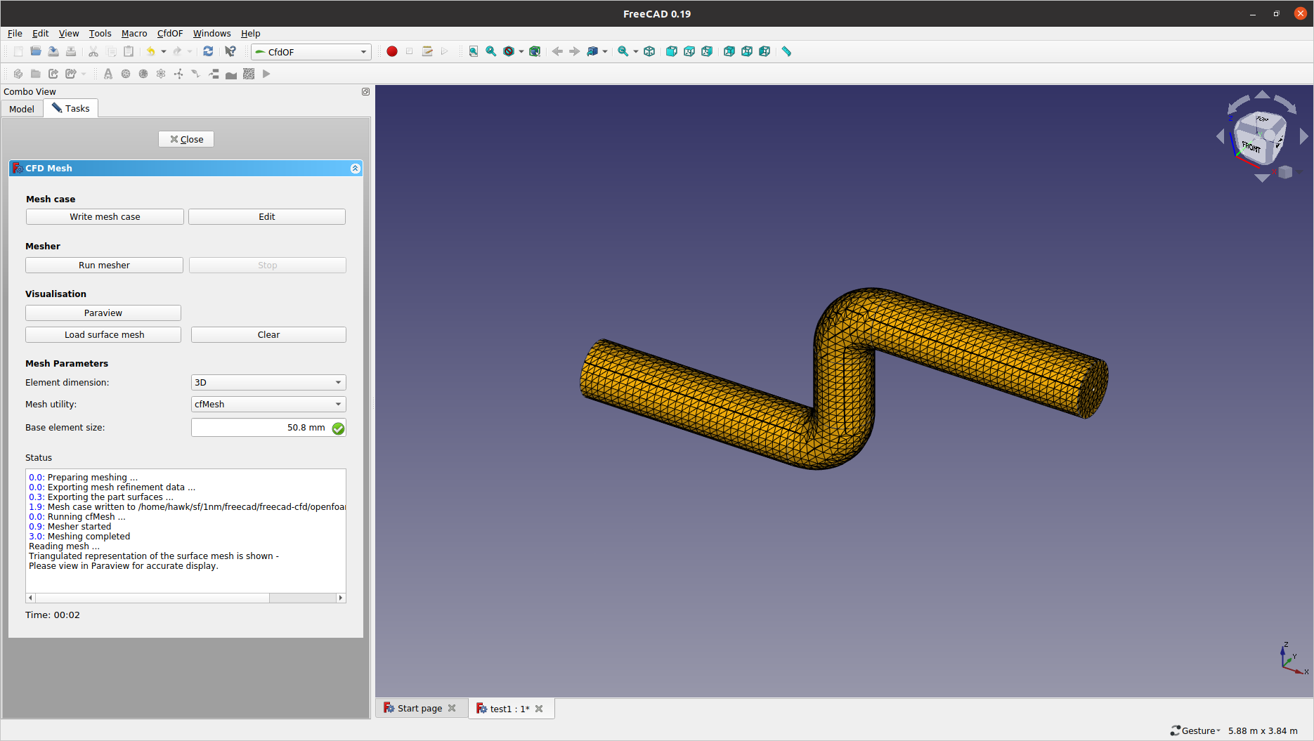
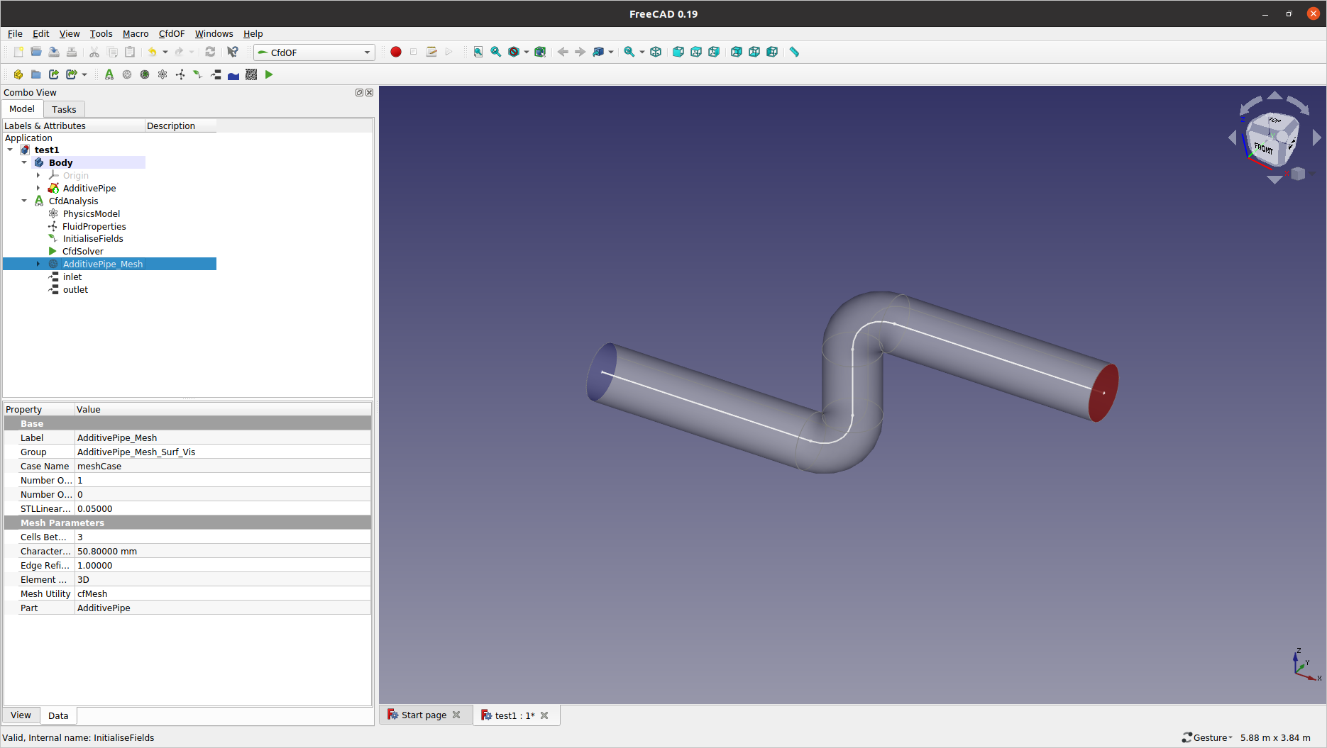
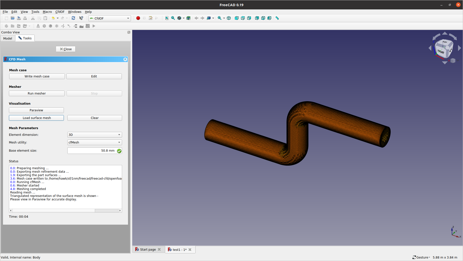
3.3: Give the Base element size value with 50.8 mm — or 0.0508 m — and click Write mesh case again. Then, click the Run mesher button to generate a preliminary mesh. When the meshing job is complete, check the surface mesh distribution by the Load surface mesh button.
-
See that the
CFD Meshpanel reported with theMeshing completedmessage. -
The base element size here is determined expecting roughly 10 cells across the pipe diameter (318 mm / 10 = 31.8 mm) after the mesh refinement (75% reduction) in the later steps (i.e. 31.8 mm / 0.75 = 50.8 mm).
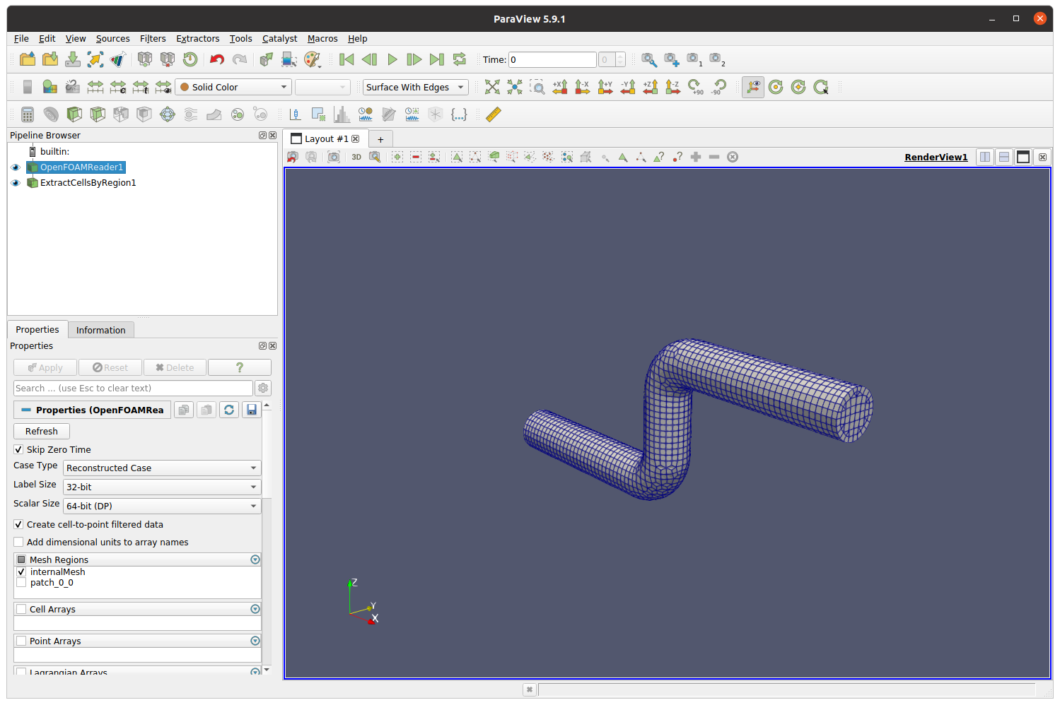
3.4: Note that the surface mesh visualisation is just a "triangulated" representation (i.e. NOT the real mesh elements). To examine the actual mesh structure, you better use ParaView by the Paraview button. We will refine the mesh after we assign boundary conditions, so for now, exit from the mesher by clicking Close.
-
If pressing
Paraviewfails in loading your version of ParaView, you can open the 'meshCase' folder manually by theEditbutton, and then start a teminal from in there to launch ParaView byparaview --data=pv.foam &.
4: Physics & materials setup
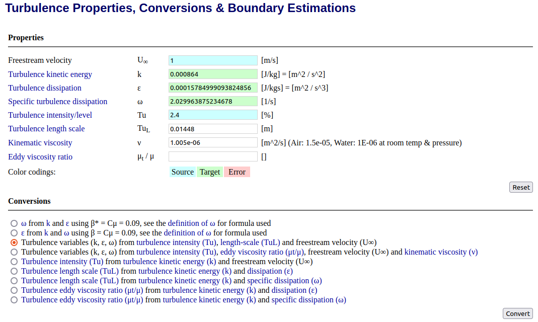
The physics involved in this exercise is chosen arbitrarily with the flow Reynolds number (based on the pipe diameter) being at 3.8 x 10⁵. Relevant turbulence modelling parameters can be easily estimated using online tools such as one provided by CFD Online.
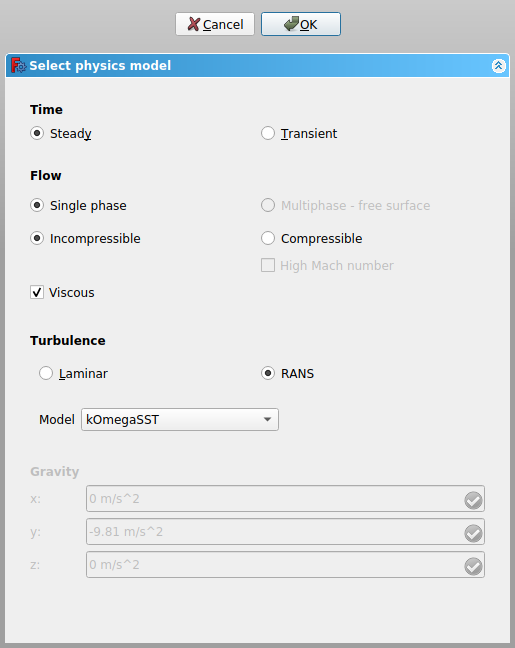
4.1: In the model tree, expand the CfdAnalysis branch to reveal the objects under it. First, double-click the PhysicsModel object to enable the Viscous and then the RANS turbulence options. Click OK to confirm.
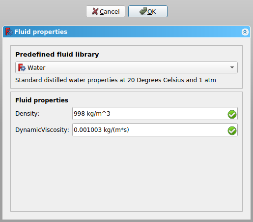
4.2: Double-click the FluidProperties object in the model tree, and select Water from the Predefined fluid library. Accept the default values for the Density and the DynamicViscosity values, and then click OK to close.
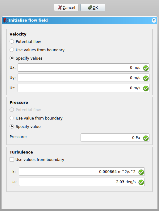
4.3: Double-click the InitialiseFields object in the model tree. Enable Specify values for Velocity and leave the values of 0 m/s in the Ux, Uy, and Uz fields. Similarly, tick on the Specify value option for Pressure with the default value 0 Pa. For the turbulence parameters, feed the following values:
-
\(k\): 8.640e-4 (m2/s2)
-
\(\omega\): 2.030 (1/s)
Click OK to confirm.
-
Note the \(\omega\) unit in the FreeCAD panel is incorrectly showing as
deg/sbut will be taken as1/son writing the input (thus, no need to convert).
5: Boundary conditions
In this example, we will assign 1 m/s of inflow from the left end which exits through the right end.
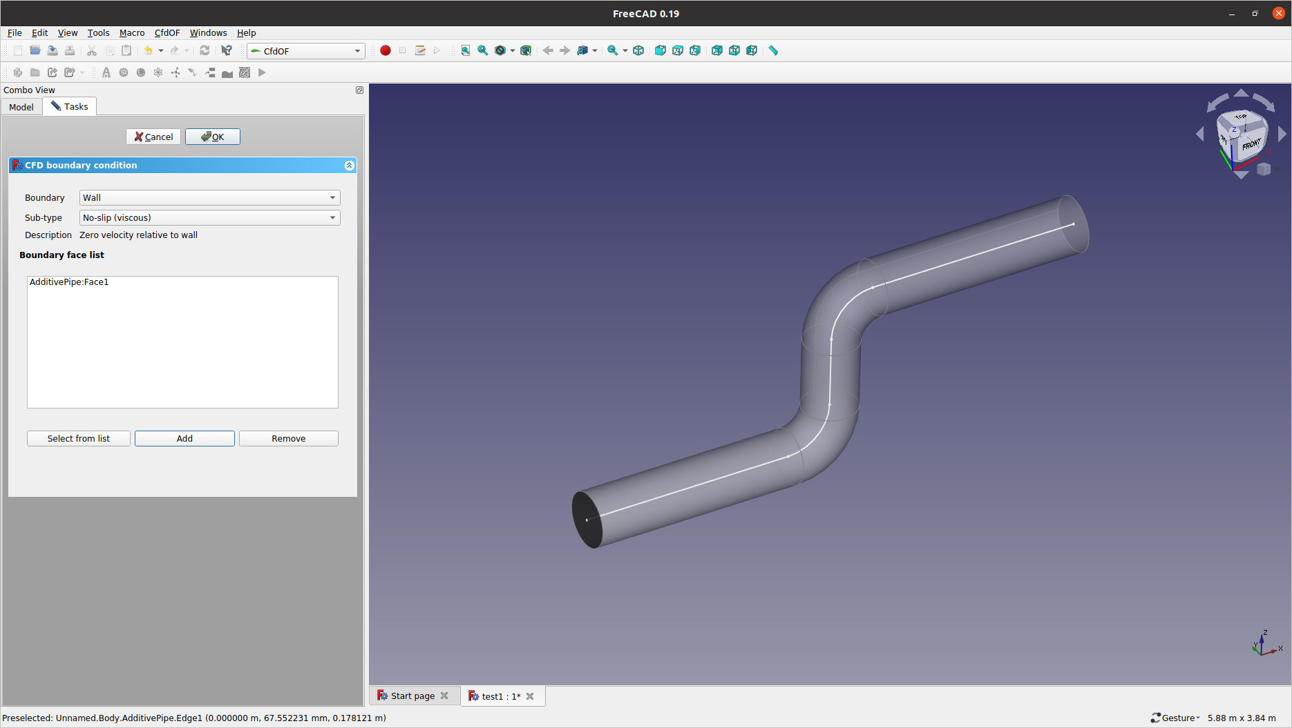
5.1: Click ![]() (
(Create a CFD fluid boundary) to define the velocity inlet boundary. Rotate the view angle so that you can pick the left cross-sectional area using the left mouse click. With the selected surface highlighted in green, click the Add button in the Tasks pane.
-
Notice the entity ID for the selected face reads like
AdditivePipe:FaceN, indicating it is the N-th face from theAdditivePipeobject.
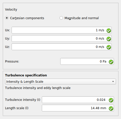
5.2: Change the Boundary type to Inlet, and then enter the value of 1 (m/s) for the Ux field. Select the Intensity & Length Scale option for the Turbulence specification and feed the same values as for the initial field ones:
-
Turbulence intensity:0.024 -
Length scale:0.01448 m(or14.48 mm)
Click OK to confirm.
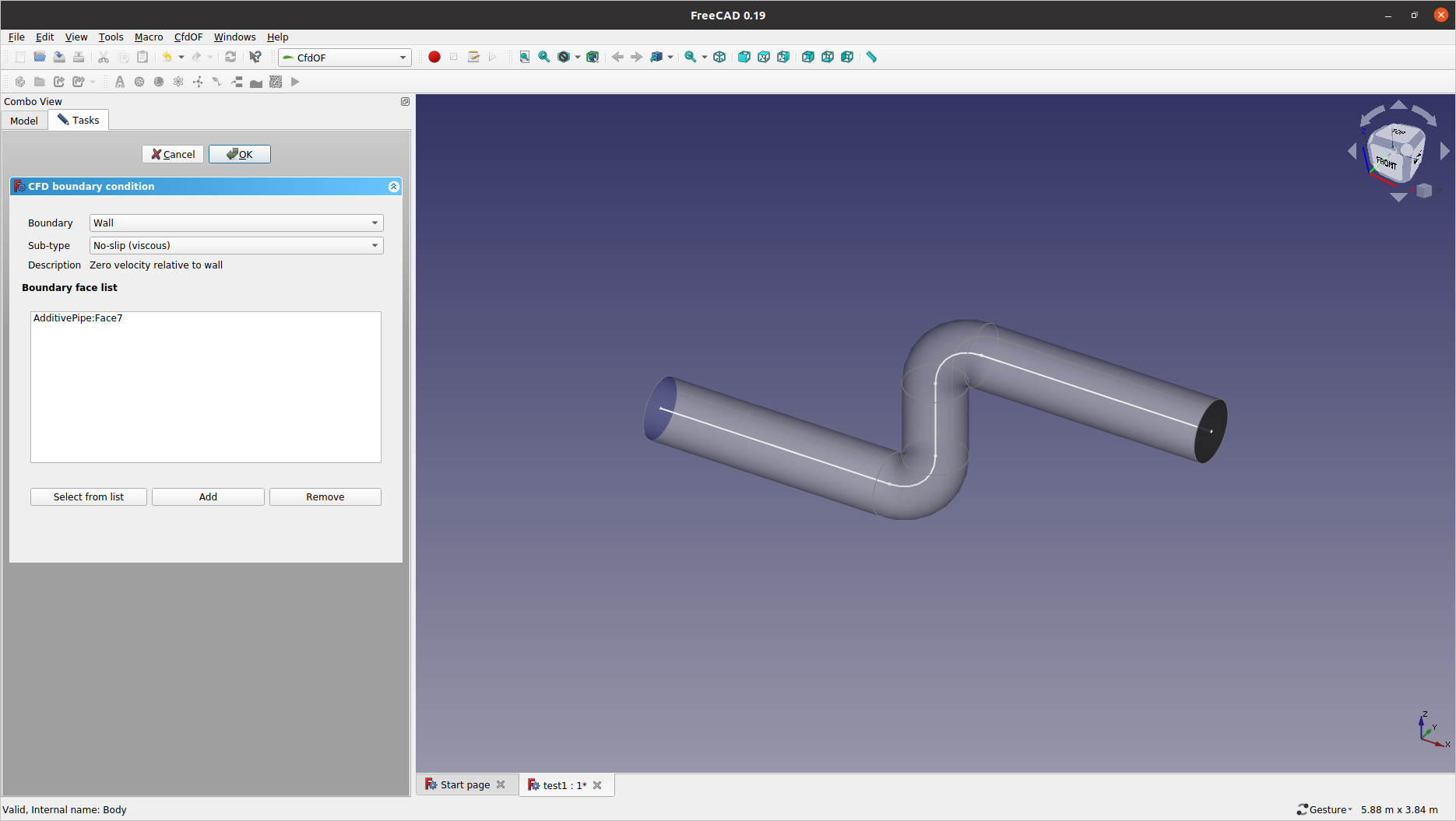
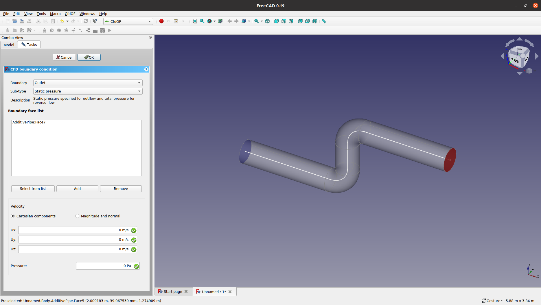
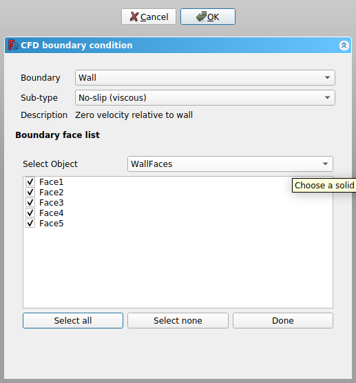
5.3: Similarly, we will assign the pressure outlet boundary condition, but this time, click the opposite cross-sectional area first and then click the ![]() (
(Create a CFD fluid boundary) icon. This will open the CFD boundary condition panel with the Boundary face list filled accordingly.
5.4: Change the Boundary type to Outlet and leave the remaining parameters as they are. Click OK to confirm.
5.5: We might continue on selecting all other faces to define a no-slip "wall" boundary condition. But doing so makes picking the same faces for boundary layer generation a bit tricky. Instead, we better handle this in the Boundary wall treatment section.
-
If you choose to add the wall boundary condition in this stage, make sure to turn the visibility off for the resulted
wallobject so that it may not hinder the same faces from being selected in the next step.
6: Boundary wall treatment
In this section, we make use the inherent mesh refinement functionality as a way to group target wall region(s) for assigning appropriate refinement strategy.
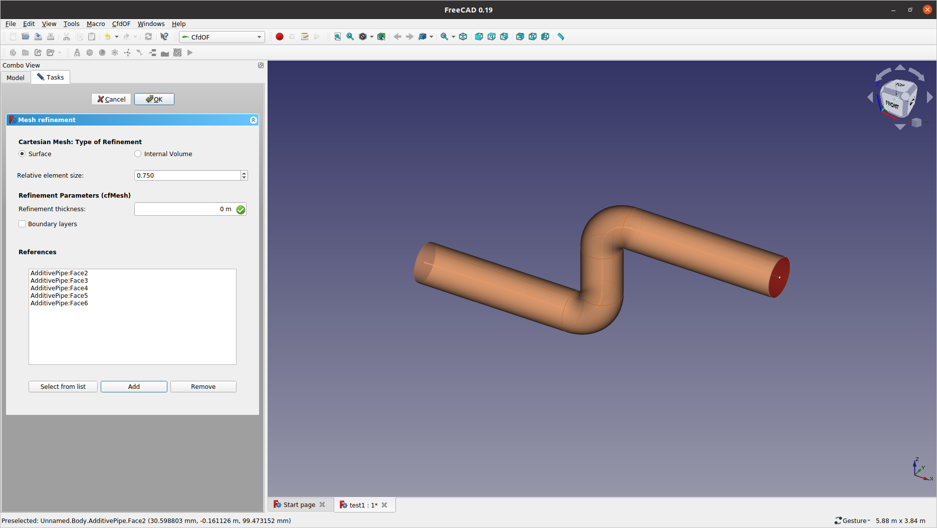
6.1: Select the main mesh object — i.e. the one labelled as AdditivePipe_Mesh in this example — and then click the ![]() (
(Create a mesh refinement) icon.
6.2: Pick the five (5) wall faces from the graphics, and then click the Add button in the Mesh refinement panel to add them to the References list.
-
If FreeCAD resists to fill the
Referenceslist with the selected faces, you may instead get them bySelect from listfor theAdditivePipeobject and then exclude the two (2) faces for Inlet and Outlet accordingly.
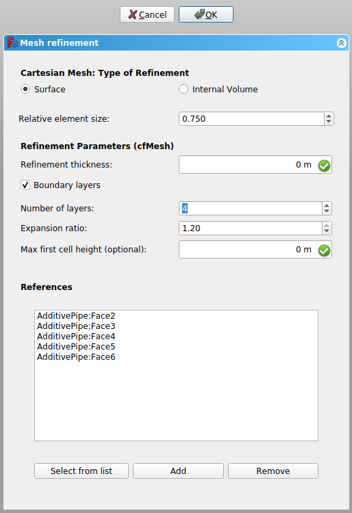
6.3: Tick on the Boudanry layers option from the Mesh refinement panel and increase the Number of layers to 4. Leave the other as they are and click OK to close.
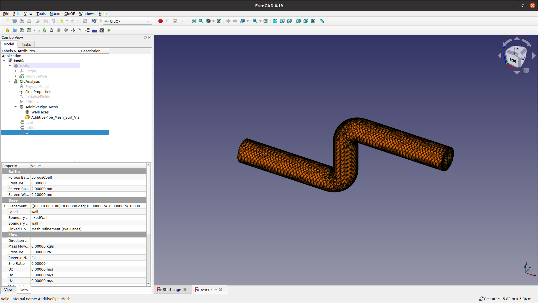
6.4: From the model tree, expand the AdditivePipe_Mesh entry and rename the MeshRefinement entry to a more intuitive name such as "WallFaces". Now, click the ![]() (
(Create a CFD fluid boundary), click Select from list, and then select the WallFaces for the Select Object list control. With all the five (5) faces selected, click OK. Turn the visibility off for the newly created wall object in the model tree.
-
Notice the previous
AdditivePipe:Face2toAdditivePipe:Face6entities are now referenced byWallFaces:Face1toWallFaces:Face5respectively.
7: Remeshing
With the boundary mesh generation parameters, we need to revisit the meshing task.
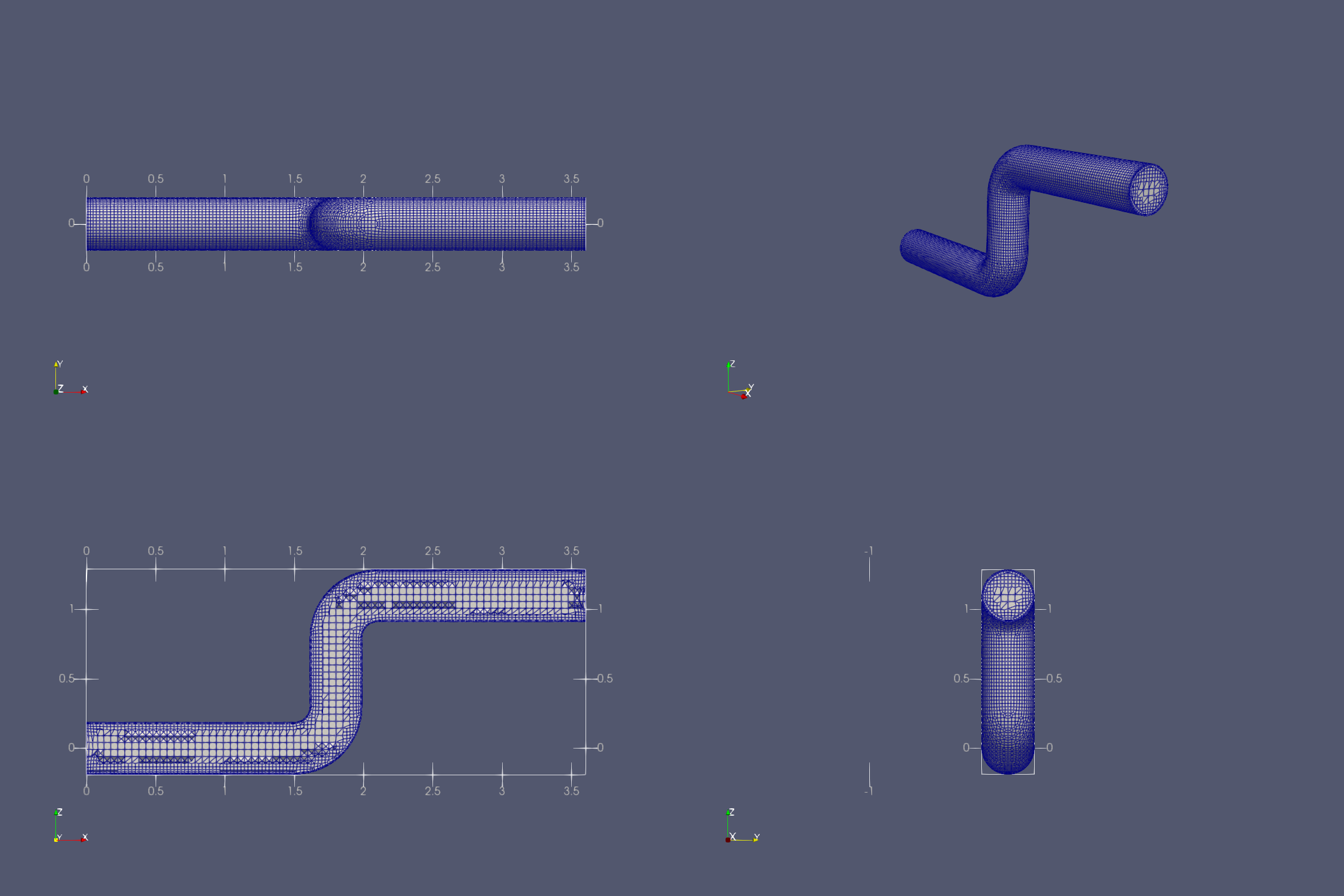
7.1: Double-click AdditivePipe_Mesh in the model tree. Initiate by clicking the Write mesh case button, and then click Run Mesher. When the meshing job is done, quickly check the surface mesh distribution by Load surface mesh.
7.2: You may launch ParaView to examine the actual mesh structure — i.e. either by the Paraview button (if it works) or by launching one manually (See Step 3.4). After a brief investigation, exit from ParaView. Also, exit from the meshing panel by clicking Close.
7.3: Note the FreeCAD changes the visibility status for individual objects as necessary. That said, you may turn on/off their respective visibility any time. It is also a good idea saving the FreeCAD document before we continue on to solving.
8: Solving
Now with the geometry and mesh ready, you can go on to solve the model using the OpenFOAM solver.
8.1: Double-click the CfdSolver object in the model tree and instantiate the case data by clicking the Write button. This constructs the 'case' folder in your work folder with the set parameters.
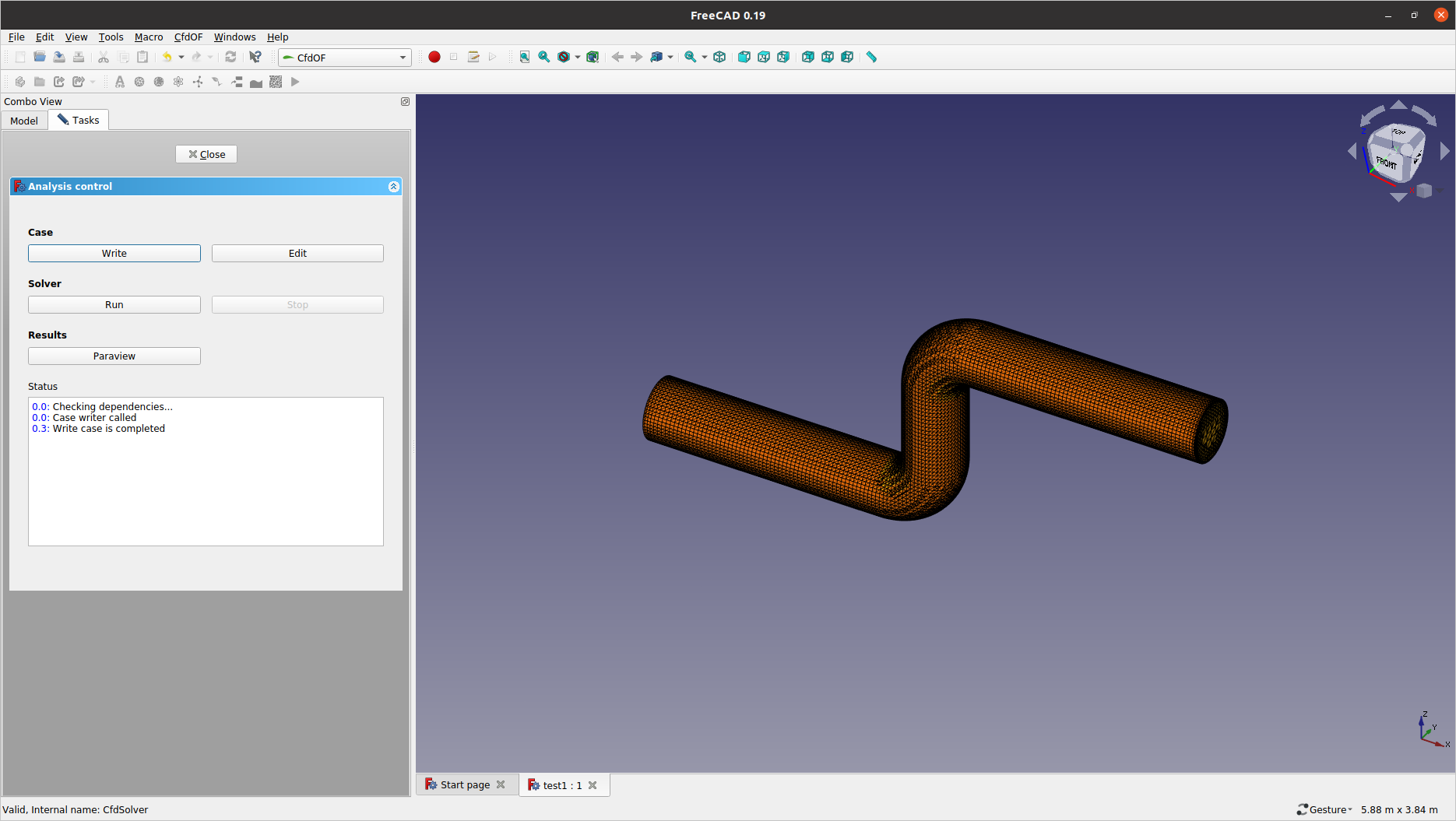
-
If you made changes any of the modelling parameters, make sure to click the
Writebutton so that it reconstructs the case folder accordingly.
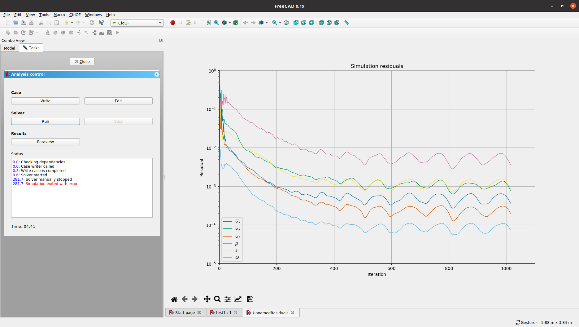
8.2: Click Run and monitor the residuals from the plotting window. Convergence seems to get stalled and wavy after around 500 iterations (possibly due to flow transient). Stop the run after around 1000 iterations.
9: Post-processing
Unfortunately, the Analysis control panel is not fully implemented for handling solved data yet. You have to navigate to the case folder and complete the remaining post-processing tasks.
9.1: Click the Edit button to open the case root directory.
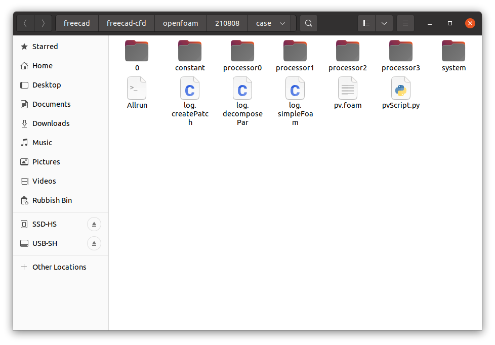
9.2: Open a terminal by right-mouse-clicking to select Open in Terminal from the context menu. For partition-decomposed cases, you first need to reconstruct the solution data using the reconstructPar command.
$ reconstructPar
Then, launch ParaView by entering:
$ paraview --data=pv.foam &
9.3: Spend some time to investigate the result by plotting pressure contours, velocity vectors, etc.