This article provides step-by-step instructions on trying out FreeCAD Workbench for FEM (Finite Element Method) on a personal computer running on Ubuntu 21.04. The FEM Workbench provides an integrated work environment for performing Finite Element Analysis (FEA) with an external FEM solver. Here, we will perform a simple computation on a cantilever beam of a rectangular cross-section using CalculiX as the FE solver.
The instructions given are for a Ubuntu 21.04 system, but it should also work for Ubuntu 20.04 and other Ubuntu-compatible distributions with Pop!_OS inclusive.
Preparation
Base components
1: FreeCAD 0.19.x AppImage: If you don’t have FreeCAD installed, you may refer to the latest FreeCAD installation tutorial from Solvercube LearnPress (registration not required for free articles). Also check out channel videos from Solvercube Channel.
2: CalculiX 2.17 (CCX 2.17): To install CalculiX, refer to the latest CalculiX installation tutorial from Solvercube LearnPress (registration not required for free articles). Also check out channel videos from Solvercube Channel.
3: Gmsh 4.8.x: Refer to the latest Gmsh installation tutorial from Solvercube LearnPress (registration not required for free articles).
FreeCAD configuration (for this tutorial)
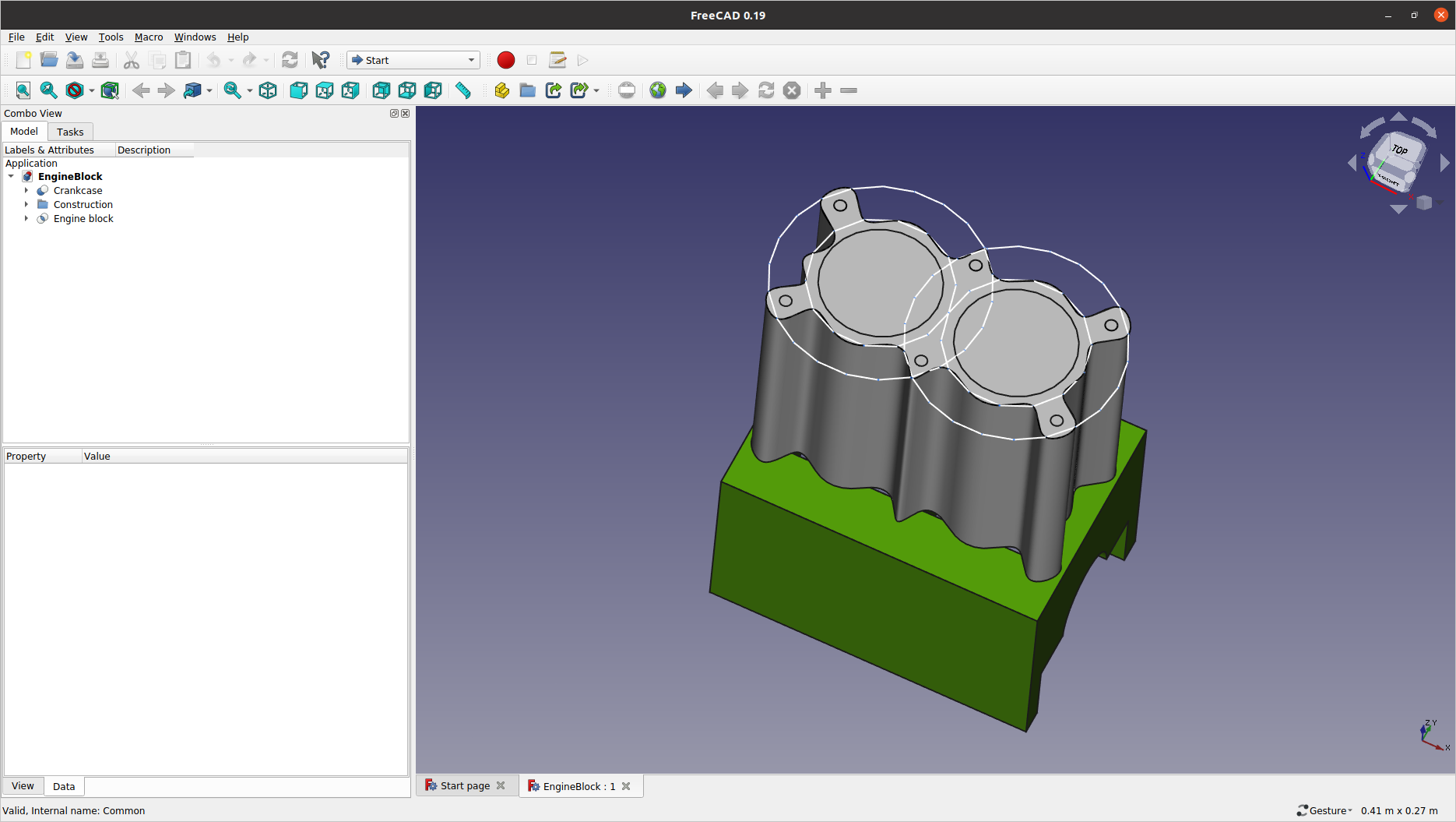
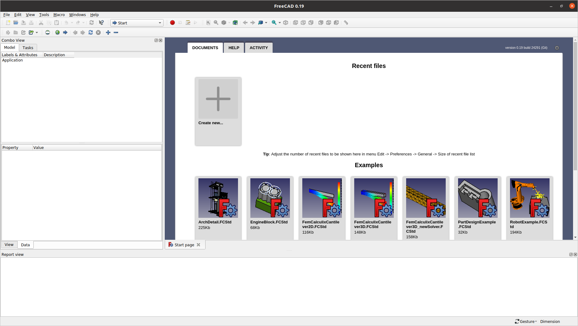
Launch FreeCAD, and open one of the example models from the Start page. Right-click on the graphics screen to select . Under this scheme, mouse operations are as follows:
-
Left button clicks on a geometrical entity: selects a single entity (e.g. a vertex, an edge, a face, etc.)
-
Left button double-click on a geometrical entity: selects the entity in the highest topological hierarchy (for example, the body containing a selected edge)
-
Left button pressed and moving around: rotates the view angle
-
Right button: opens the FreeCAD context menu
-
Right button pressed and moving around: moves the viewport laterally (i.e. panning)
-
Middle mouse click over a geometrical entity: centres the viewport around the clicked entity
-
Mouse wheel: zooms in and out the viewport, with the current cursor point being the scaling origin
You can also control the viewport using the Keyboard Navigation keys:
-
Ctrl++ and Ctrl+-: zooms in and out, respectively
-
The arrow keys, ◄ ► ▲ ▼: shifts the viewport left/right and up/down, respectively
-
Shift+◄ and Shift+►: rotates the view angle by 90 degrees around the screen’s normal axis (i.e. z-rotation)
-
The numeric keys, 0 1 2 3 4 5 6: there are seven (7) pre-defined views, that are, Isometric, Front, Top, Right, Rear, Bottom, and Left.
-
Pressing V then F: sets the viewport to fit the visible object(s)
-
Pressing V then O: sets the camera in Orthographic view
-
Pressing V then P; sets the camera in Perspective view
-
Pressing and holding Ctrl: allows you to select more than one entity (i.e. multiple selections).
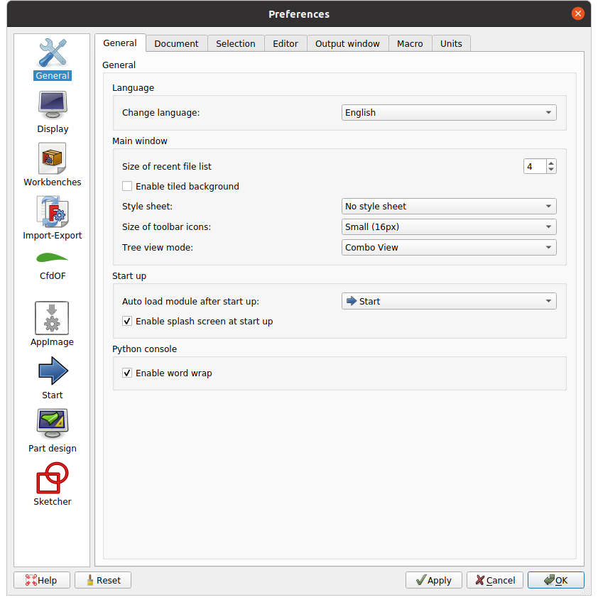
Note that FreeCAD GUI (Graphical User Interface) has many toolbar icons to boost productivity. I suggest reducing the toolbar icons size so that more icons be visible at once: Visit the menu, and select Small (16px) for the Size of toolbar icons (from the Main window section).
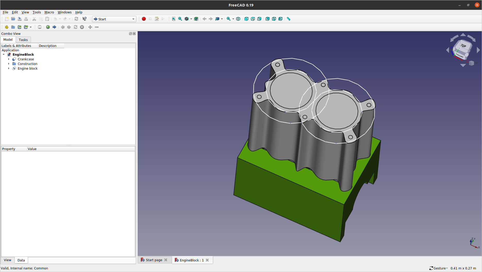
Also, from the main GUI layout, relocate the View toolbar
from the default position (the forefront of the second row) to the rear end of the first row. It will leave more space spared for the workbench tools we are going to use in this tutorial.
FEM Workbench Exercise
We will build the geometry from the Part Design Workbench and then switch to the FEM Workbench for the stress analysis on the geometry.
1: Part Design Workbench
Start FreeCAD from a local work folder and select Part Design from the workbench selector (currently showing as ![]() ).
).
1.1: Click the ![]() (
(Create a new empty document) icon in the toolbar area to start the Part Design module.
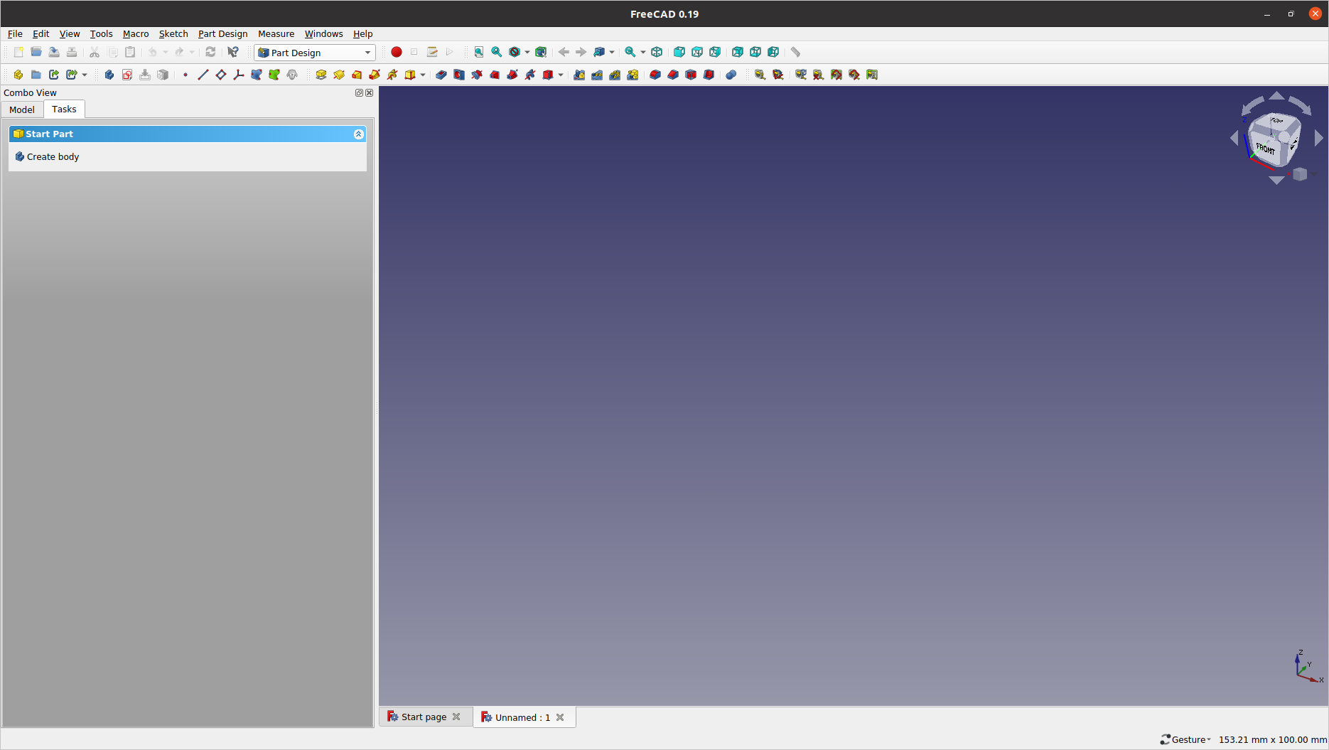
1.2: Let us close (or detach) the Report view panel from the layout for now — either using the menu or by the panel’s close button. (It will come back anyway whenever FreeCAD needs to inform you of something.)
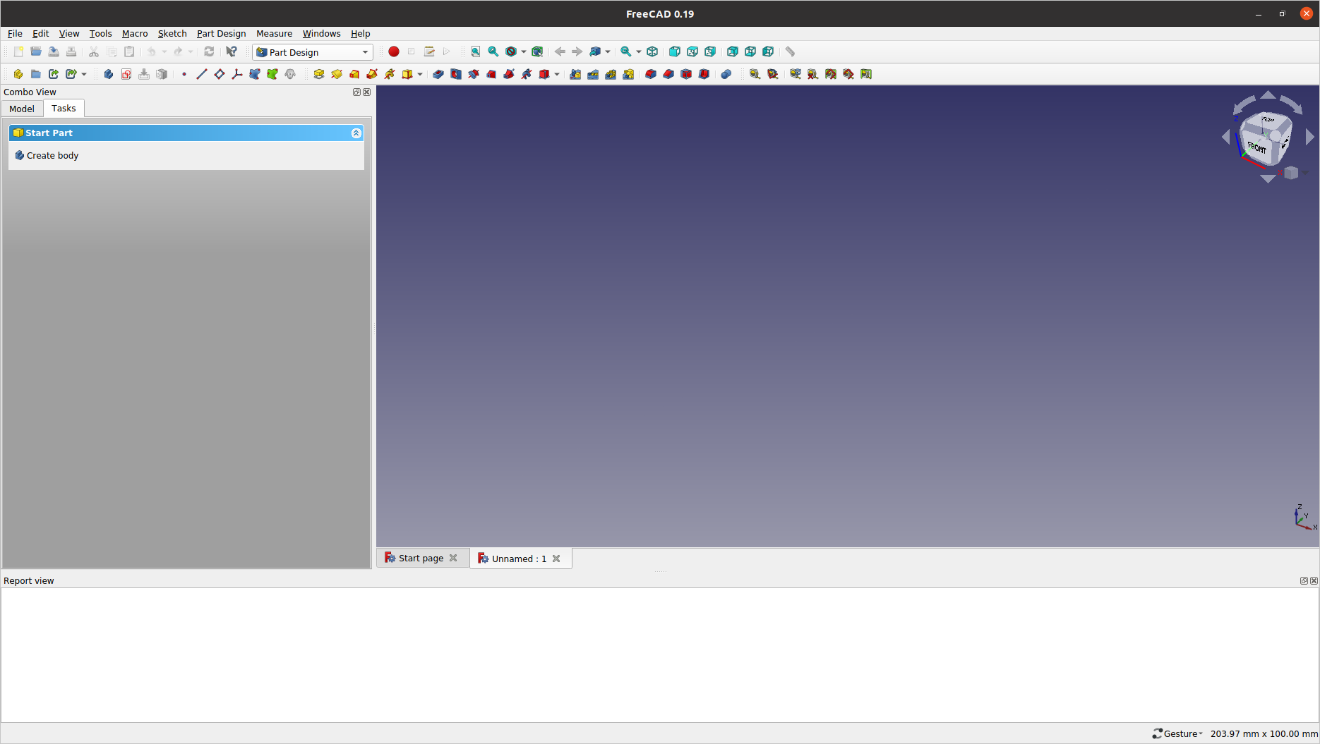
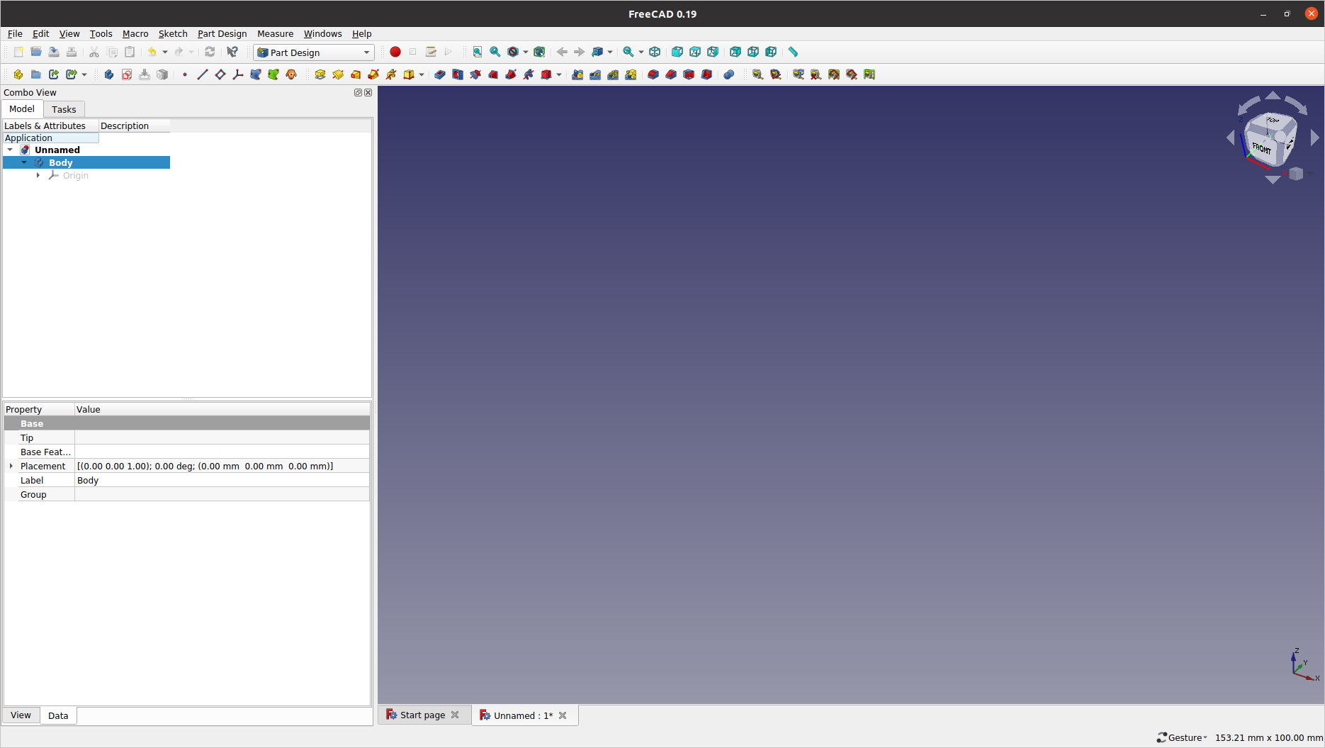
1.3: Click Create body under the Tasks tab in the Combo View panel; This area will be dubbed simply as the Tasks pane from now on — unless a specific task panel name is better mentioned.
1.4: You can see the Tasks pane now suggests follow-up actions on completing the previous task; This is a modelling wizard feature, can assist occasional users in reminding what to do next.
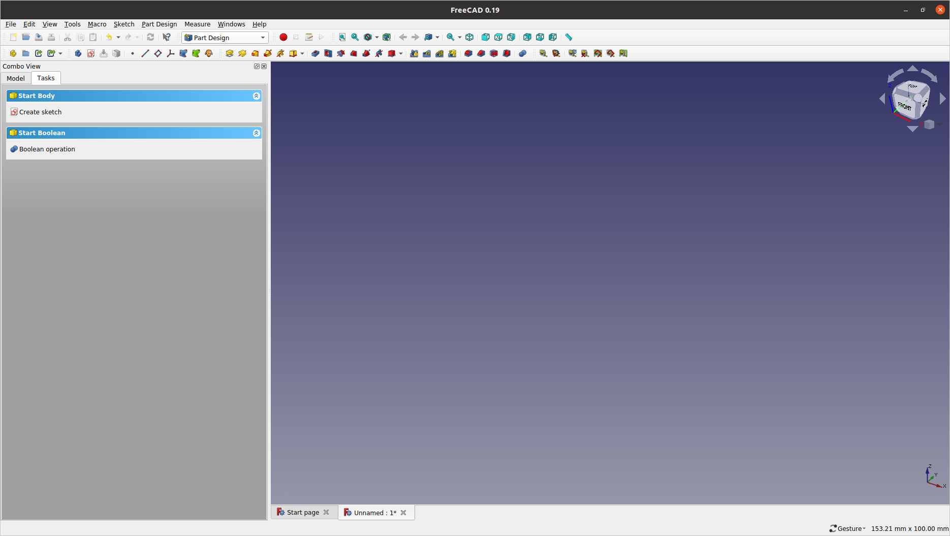
1.5: Click the Model tab from the Combo View panel to switch to the modelling tree view. See that one (and only) Body object is added under the Unnamed document root. Click the ![]() (
(Create a new sketch) icon from the toolbar to invoke the Sketcher module.
2: Sketching a cross-section
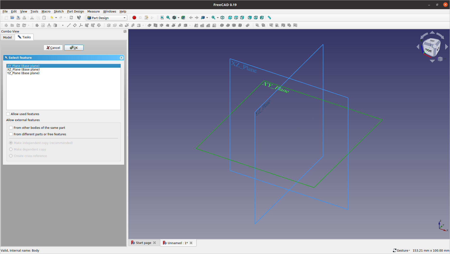
We will create a rectangular cross-section of 50 mm x 50 mm in size on the XY Plane.
2.1: Select XY_Plane either from the graphics area or the list shown in the Tasks pane. Click OK to confirm the plane selection.
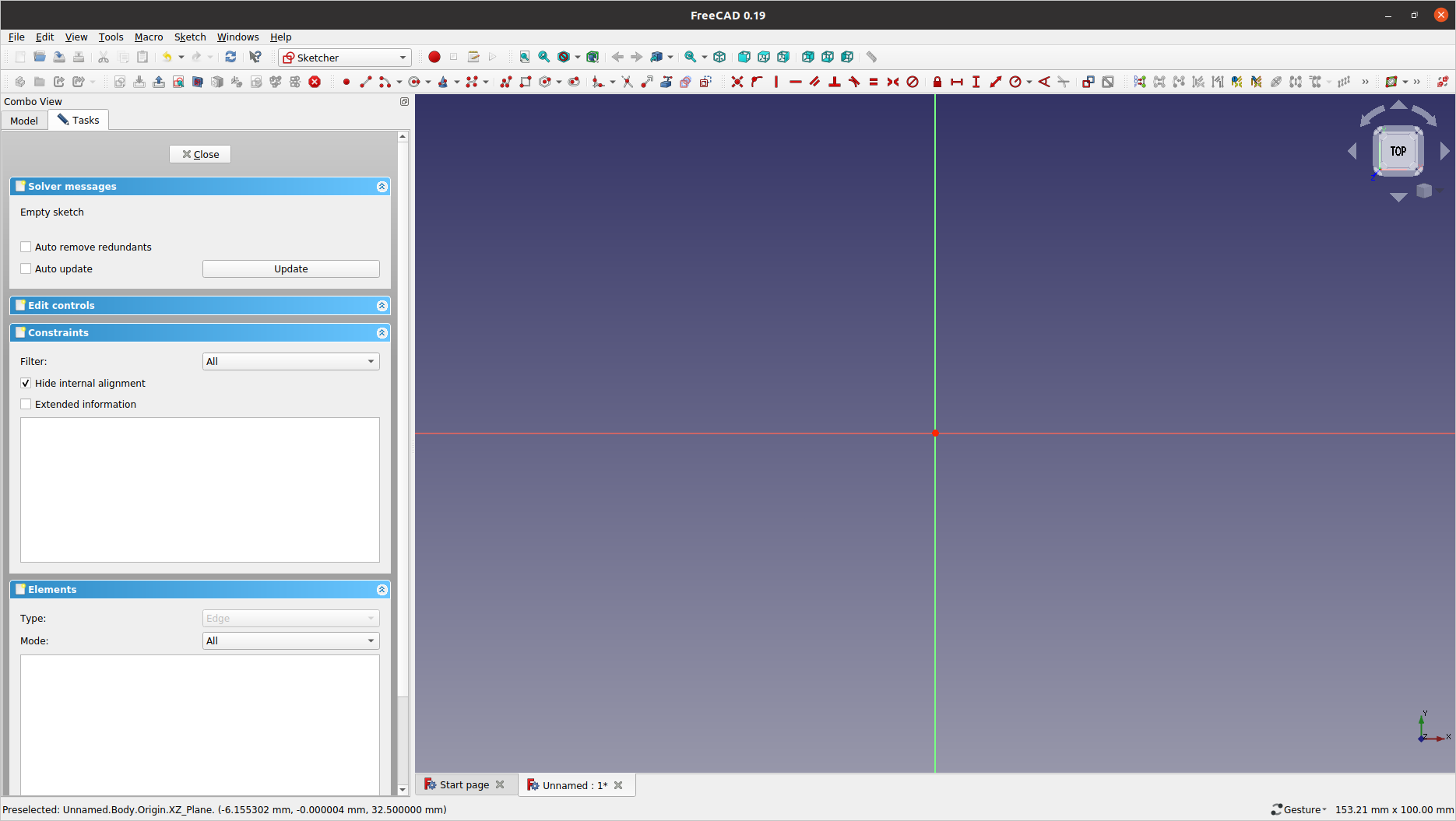
2.2: You now have entered the Skecher mode and the graphics viewport has turned into a 2D sketch pad.
-
While you are in the Sketcher mode, try moving around the viewport laterally with the mouse right-button pressed and holding.
-
Casual click of the right-mouse button opens a modelling context menu, which provides a shortcut to individual sketching tasks. This will become handy as you get accustomed to using FreeCAD.
-
Pressing and holding the right-mouse button longer than a second and then releasing it will open the context only with graphics view control functions in the menu.
2.3: Click the ![]() (
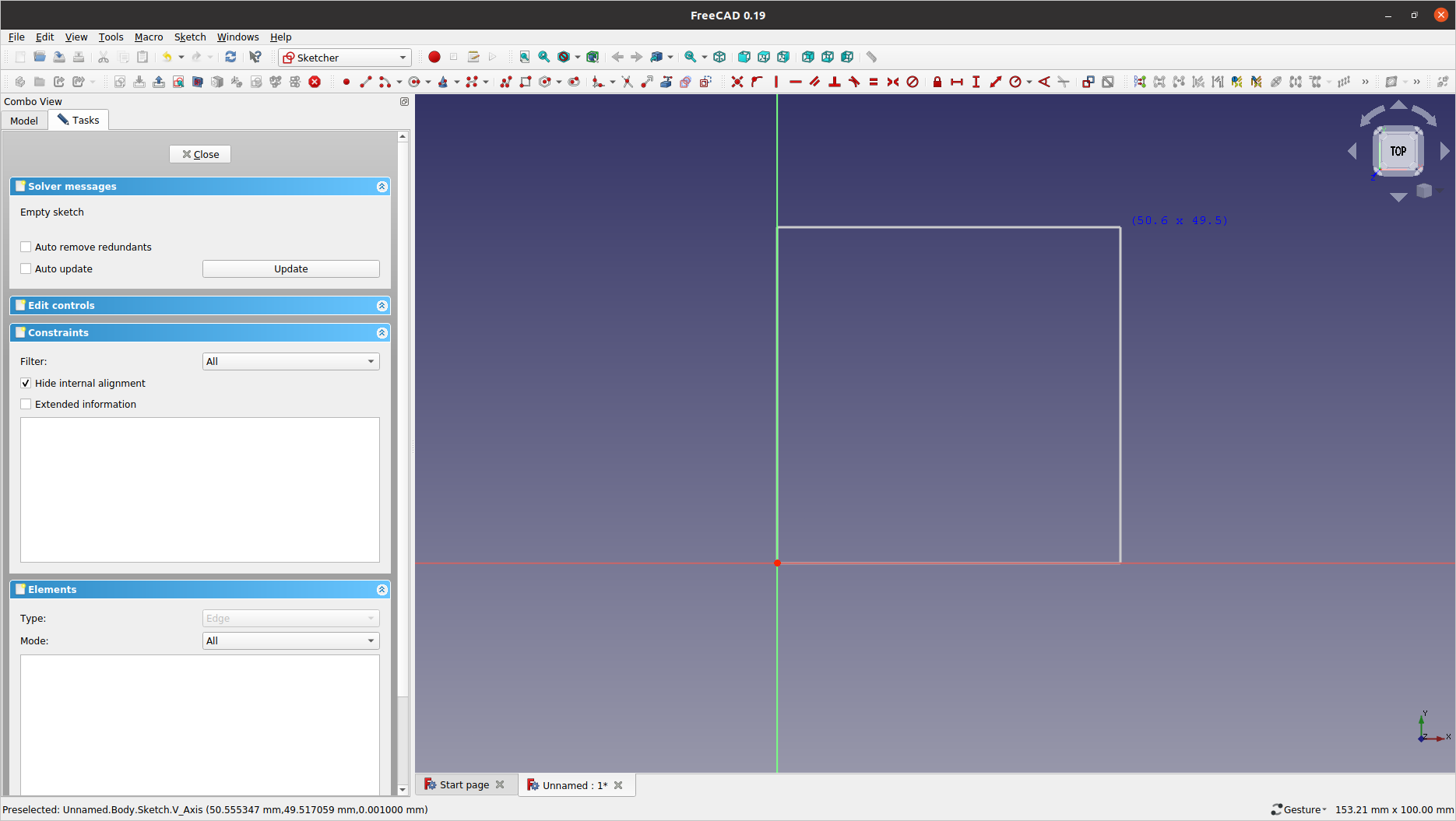
(Create a rectangle in the sketch) icon from the toolbar, and notice the change of the cursor shape indicating the current unit operation; This will be called a ghost graphic or a ghost cursor. Move the ghost cursor towards the origin point until the point colour turns to grey (this ensures establishing a coincident constraint), and make the first click to pick it as the starting anchor.

2.4: Then, move the cursor away from the origin in the +X+Y direction diagonally while monitoring the additional ghost graphic information on the dimension. On roughly sizing the wireframe, make the second click to finalise the rectangular cross-section.
-
You may get the initial sketch dimension as close as the final one by combining mouse actions of zooming in/out (using the mouse wheel), panning (with the right mouse button pressed), and viewport recentering (by clicking the middle mouse button).
-
If the result from any unit operation is not satisfactory, you can undo it by pressing Ctrl+Z to start over.
-
You can also delete any completed feature from the model tree — as long as this will not deteriorate the modelling hierarchy.
2.5: Click the ![]() (
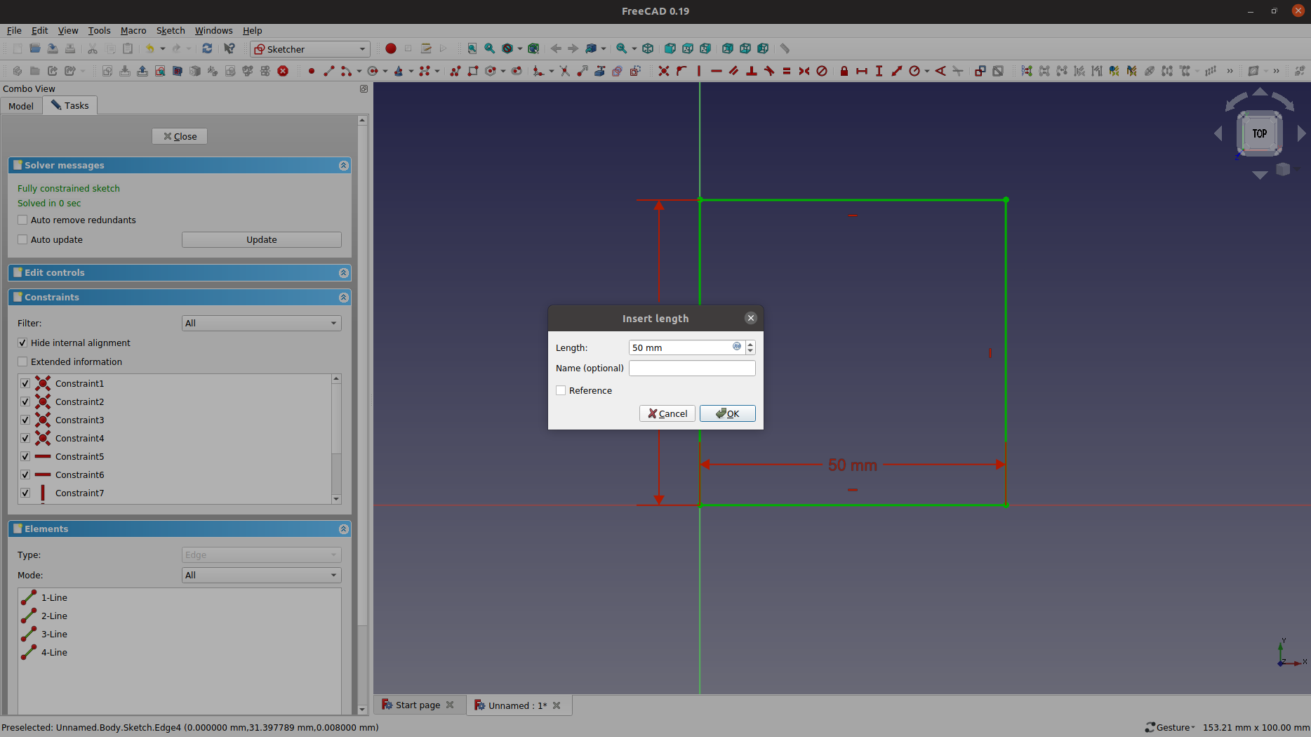
(Fix the horizontal distance) icon from the toolbar area. Hover the mouse cursor around the bottom edge and pick it when the edge colour changes accordingly. Enter 50 mm for the Length in the Insert length dialog window, and then click OK or press Enter.

-
In FreeCAD, many unit operations (e.g. drawing lines, assigning dimension values, etc) are identified by the ghost graphics attached to the mouse cursor. Clicking the right mouse button anytime ends the current unit operation returning the cursor to the normal arrow.
-
If you need to change the assigned dimensional value, check first if the mouse cursor is the normal arrow, and then double-click the target dimension either from the graphics window or from the Constraints list in the Tasks pane.
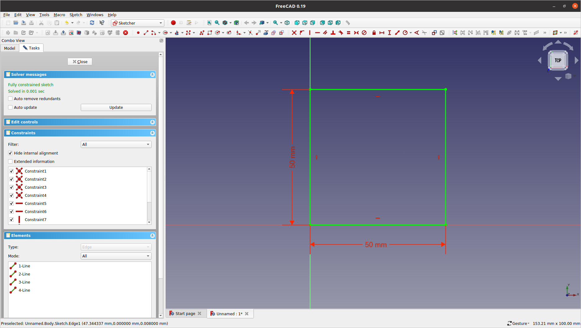
2.6: Similarly, assign the length of 50 mm to the left vertical edge using the ![]() (
(Fix the vertical distance) icon.
-
Again, right-clicking an empty spot will return your ghost cursor back to the normal arrow (i.e. the selection mode). Pressing the Esc button also works if the graphics area has the current mouse focus.
-
In the selection mode, you can select any of the dimension graphics to re-position. You may practice to move the horizontal dimensioning auxiliaries to the below of the bottom edge (as seen in the next image).
2.7: Click the Close button in the Tasks pane when done dimensioning.
2.8: You have returned to the 3D graphics mode, and the modelling tree now has a Sketch object.
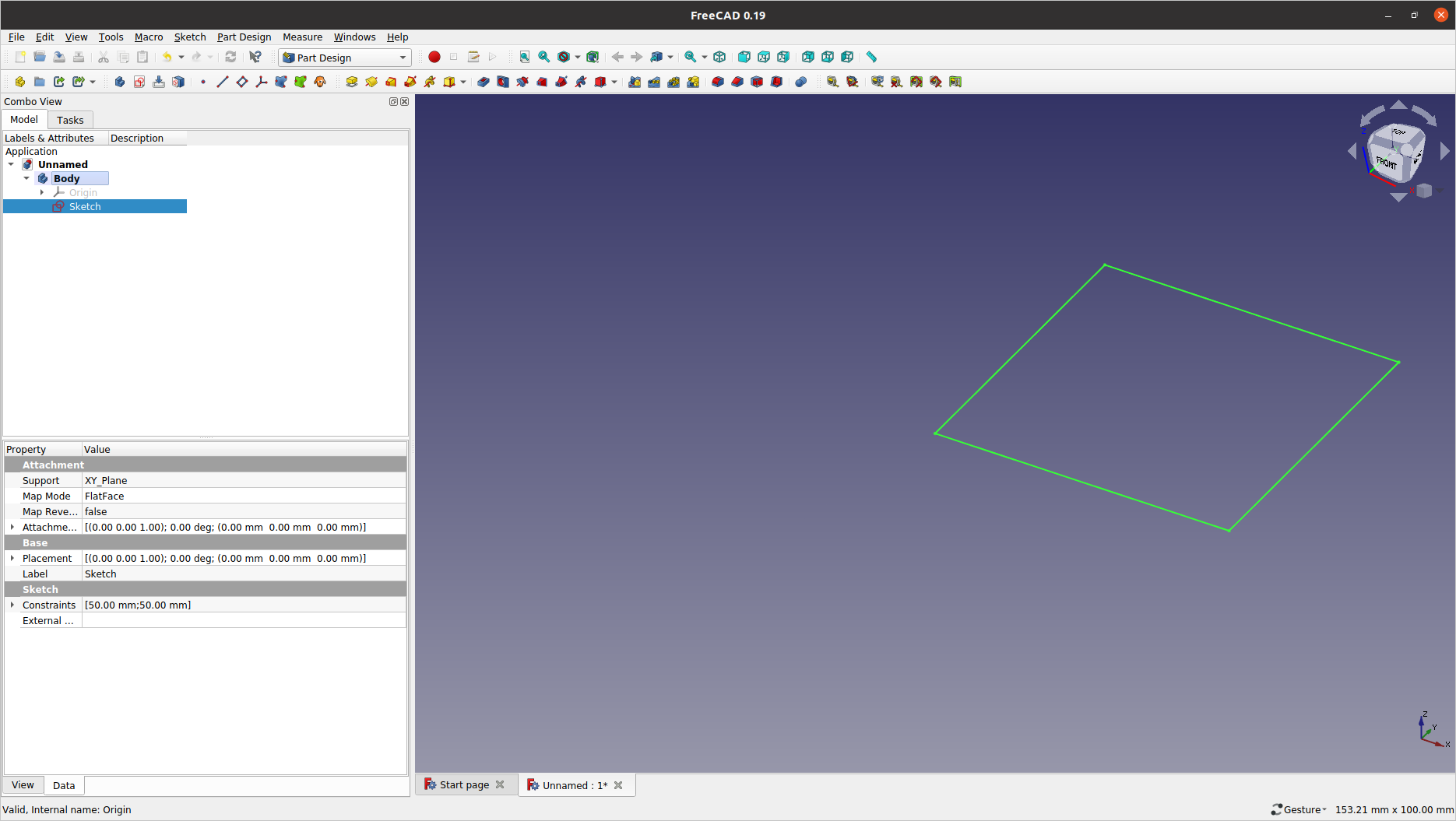
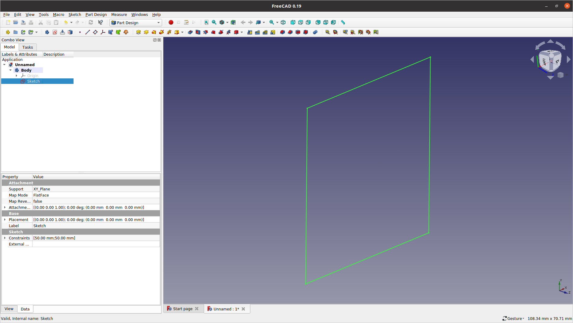
2.9: Press the numeric key 2 followed by V F to fit the viewport to the geometry. Tilt the view angle slightly using the left mouse button (pressed) before we extrude this sketch in the +Z direction.
3: Extrusion using the padding feature
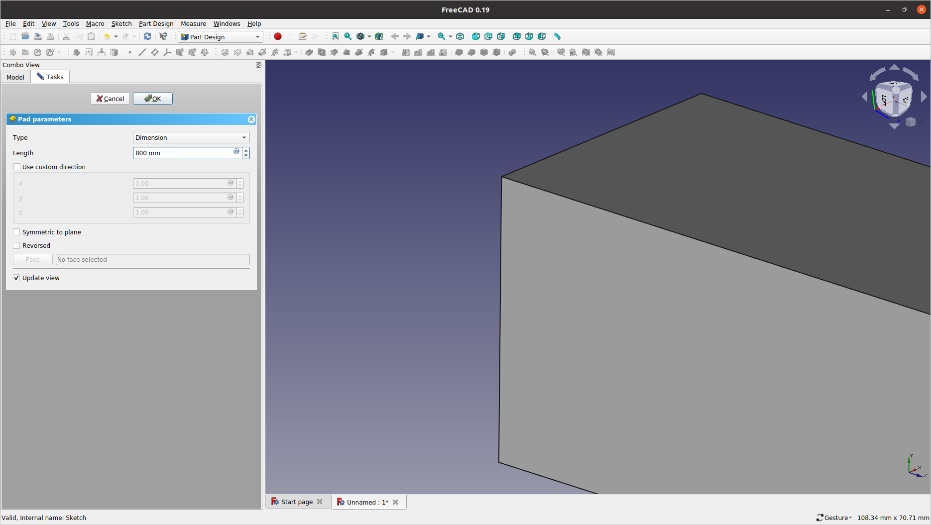
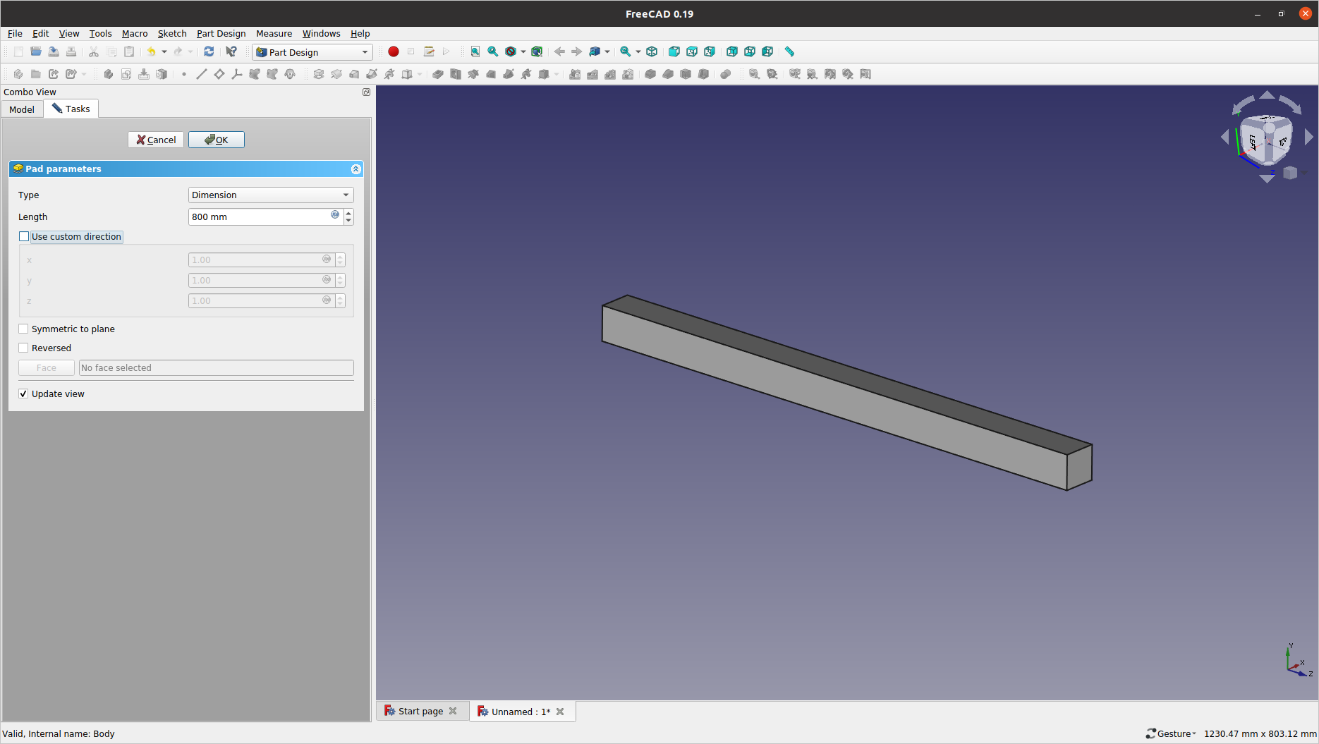
Now, we are going to extrude the sketch in the +Z direction by 800 mm to define a cantilever beam.
3.1: With the Sketch object selected in the model tree, click the ![]() (
(Pad a selected sketch) icon. Enter 800 mm — or 0.8 m — for the Length in the Pad parameters panel and then press the Tab key so that the graphics be updated accordingly. Adjust the graphics view so that the entire geometry be showing.
-
To fit the viewport to the geometry, first click an empty spot in the graphics area (to give it the mouse focus), and then press V F.
-
Alternatively, you may use the view control context menu by right-mouse clicking on an empty spot and selecting
Fit all.
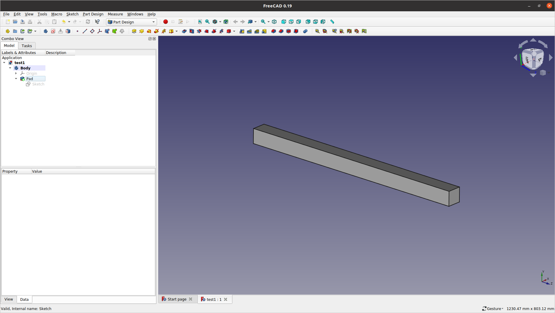
3.2: Click OK to confirm the extrusion feature.
3.3: The Body object now has a Pad feature, with the previous Sketch object relocated under it. Save the current FreeCAD document to a local work folder by before we proceed to the FEM Workbench session.
-
FreeCAD follows a conventional parametric modelling approaches. If you want to redefine the
Padfeature, just double-click the entry from the model tree to invoke its feature-editing task panel. -
If you want to start over from the base sketch, delete the
Padentry from the model tree and it will promote theSketchback to its previous position.
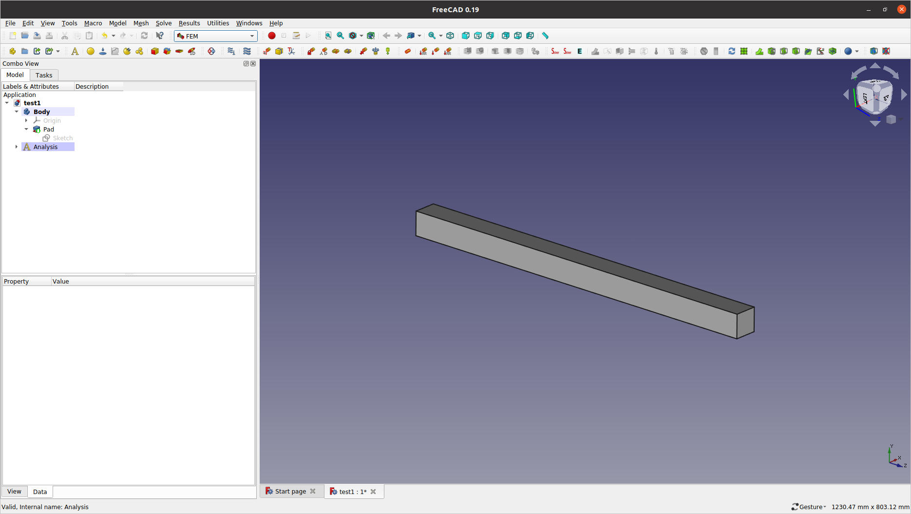
4: FEM Workbench
With the beam geometry completed, select FEM from the workbench selector to enter the FEM Workbench.
4.1: Click ![]() (
(Create an analysis container) from the toolbar. Make sure one (and only) Analysis object is created in the model tree.
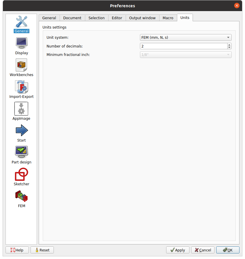
4.2: You may visit the menu to change the Unit system to FEM (mm, N, s) in the General group under the Units tab.
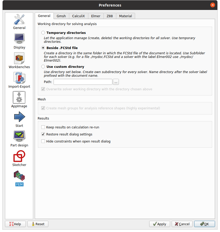
4.3: Also, visit the FEM group, go to the General tab to select where you will store the CalculiX solution files. Keep all the other settings as they are and close the Preferences dialog by clicking the OK button.
5: Material assignment
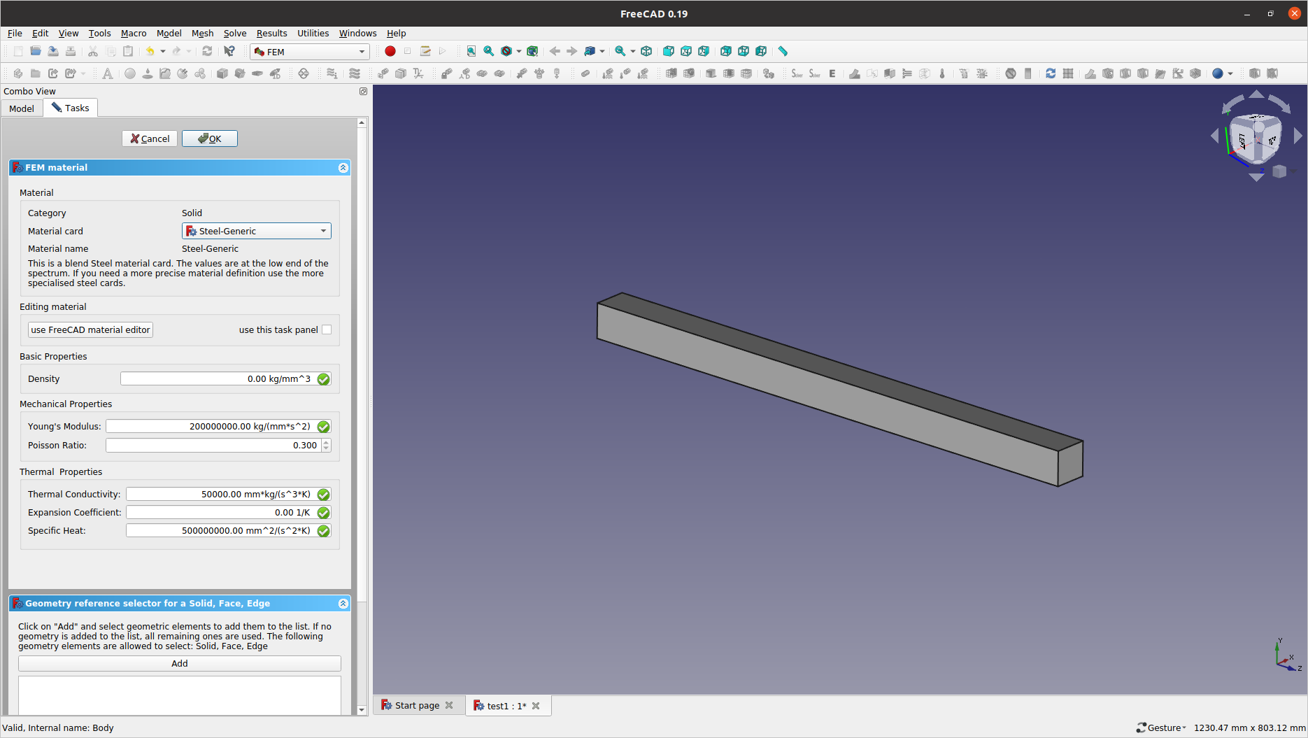
5.1: Click the ![]() (
(Create a FEM material) icon and select Steel-Generic for the Material card. Click OK to confirm.
-
In the current example, we will merely perform a static computation, thus the
Densityinput is not required.
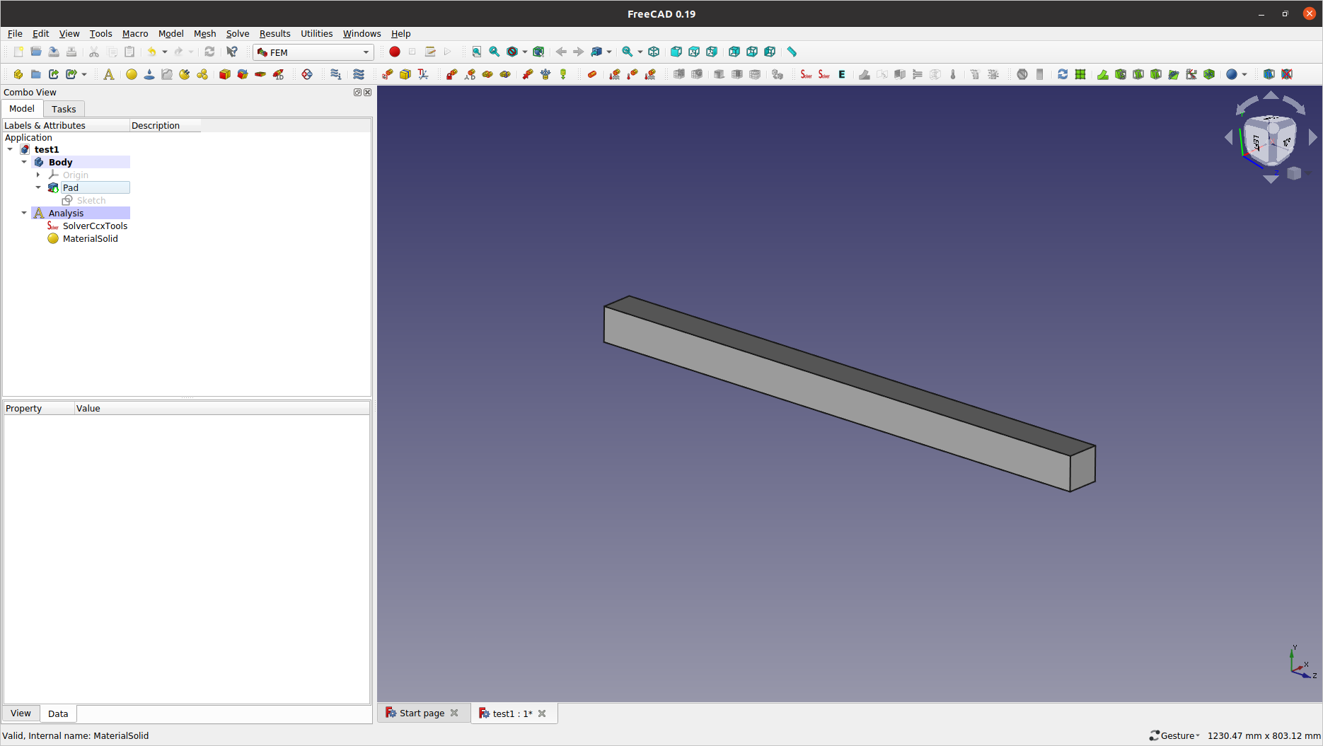
5.2: Expand the Analysis branch in the model tree to check if a MaterialSolid object is inserted.
-
Note that double-clicking any editable objects from the model tree will open the corresponding task panel. You can switch between the model tree and the Tasks pane interactively, but make sure to close any worked task panel before moving on to a "new" task.
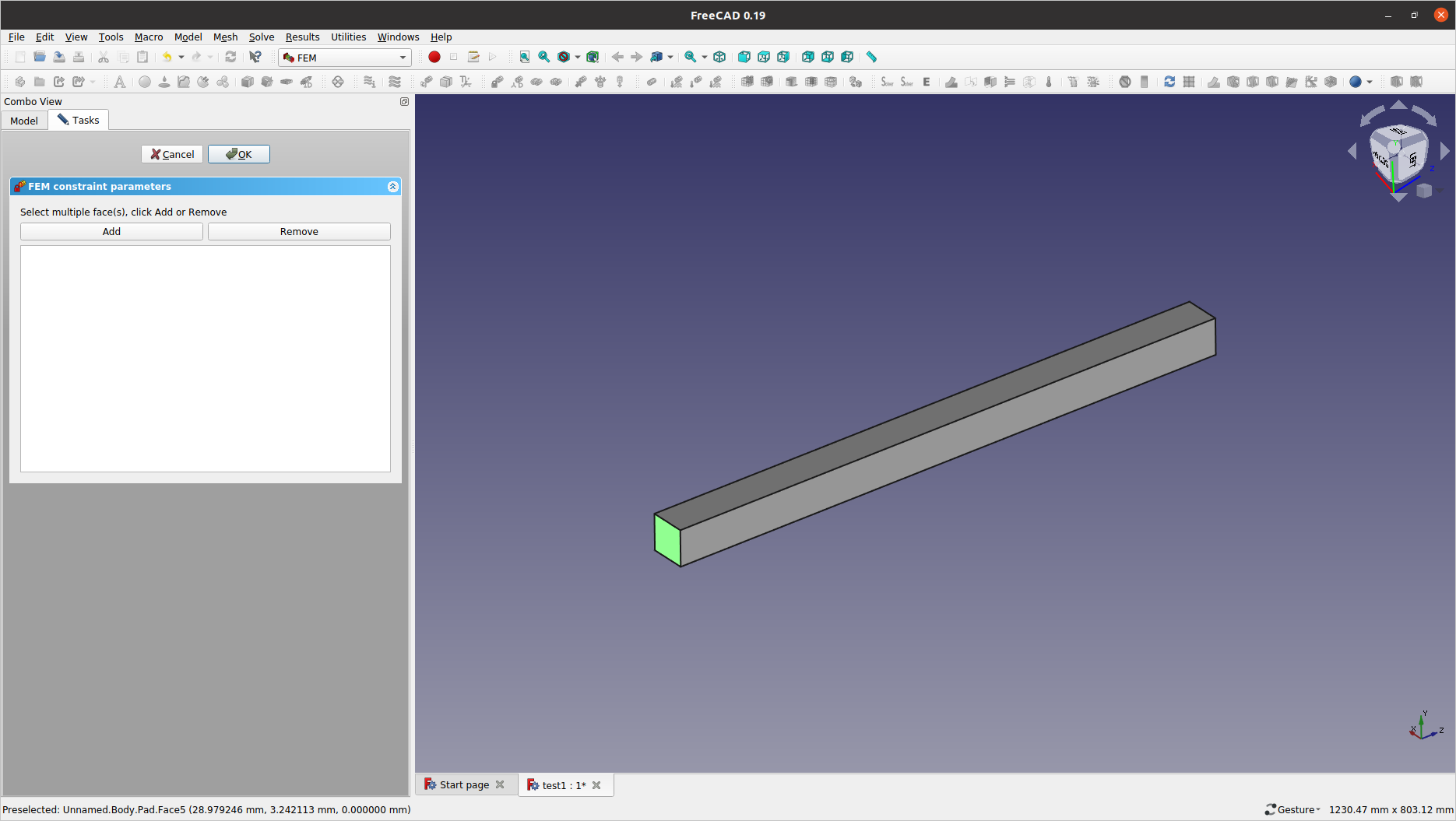
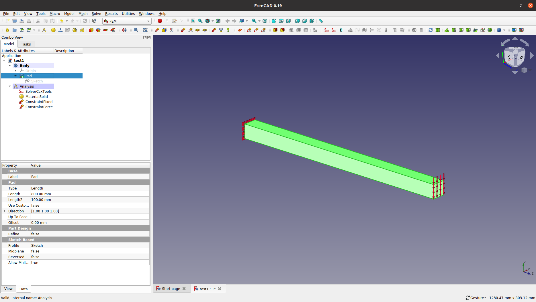
6: Boundary conditions
Here, we will fix the left end of the beam, and assign a downward force on the opposite end.
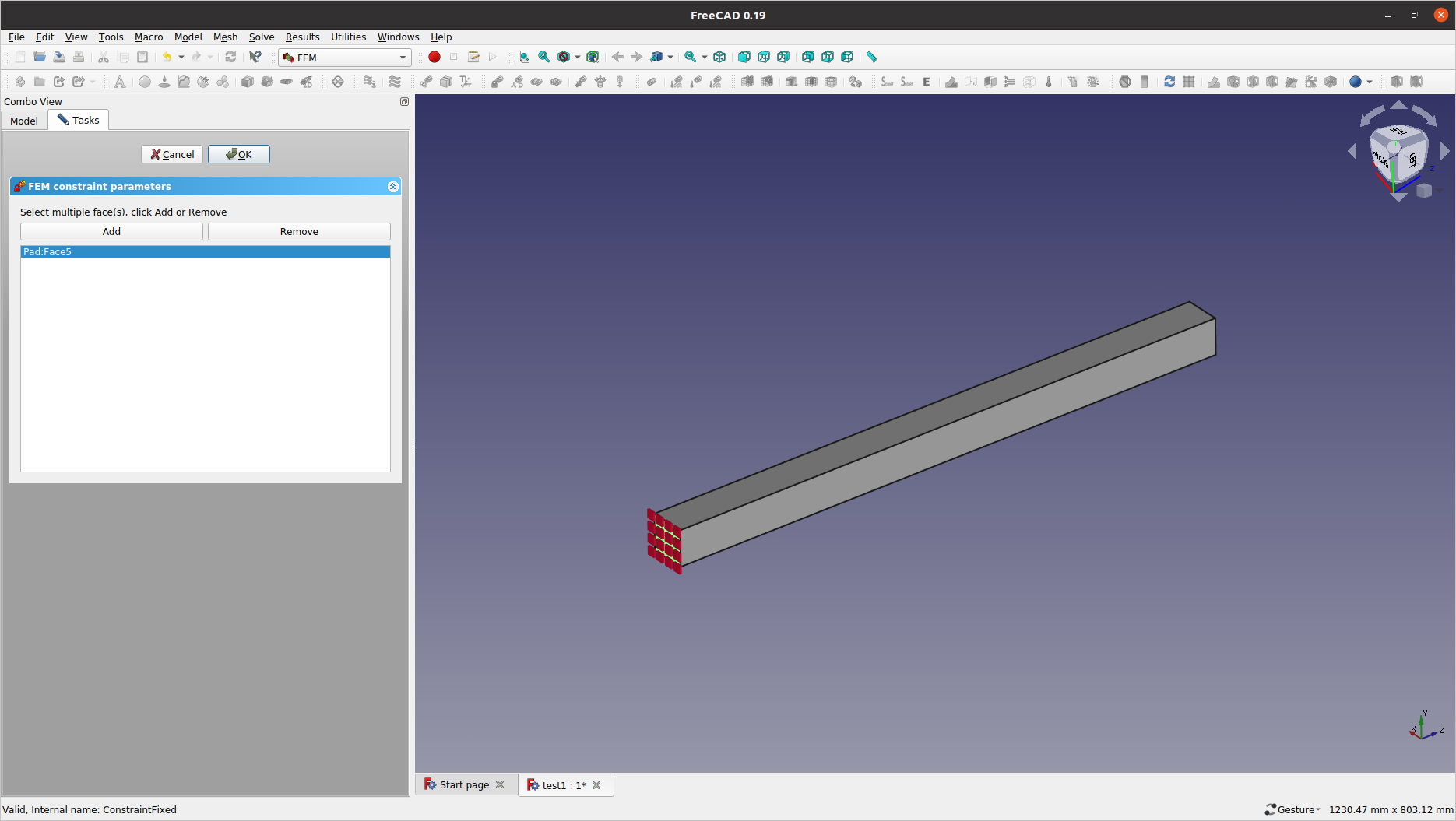
6.1: Click ![]() (
(Create a FEM constraint for a fixed geometric entity) from the toolbar. Rotate the view angle so that you can pick the rectangular face on the -Z plane. Click Add in the Tasks pane.
6.2: Click OK to complete the boundary selection.
-
If made a mistake in any setting, you can either invoke the corresponding task panel to redo, or delete the resultant object from the model tree and then start over.
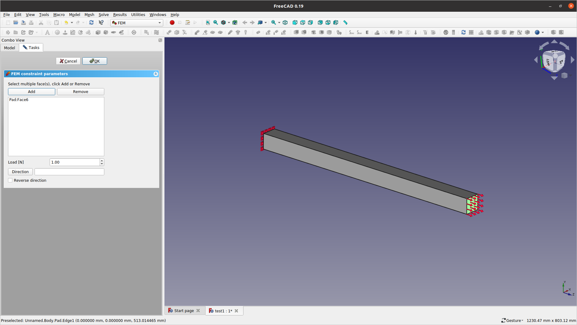
6.3: Click this time the ![]() (
(Create a FEM constraint for a force) icon. Rotate the view this time to pick the opposite end on the +Z plane. Click Add in the Tasks pane. Do NOT confirm the action yet as we need to change the direction of the applied force.
-
Alternatively, you can pick an entity (or a group of entities) first then invoke the follow-up task panel afterwards.
6.4: To assign the force in the negative Y direction, zoom in a bit (using the mouse wheel) and pick one of the two (2) vertical edges on the free-end side.
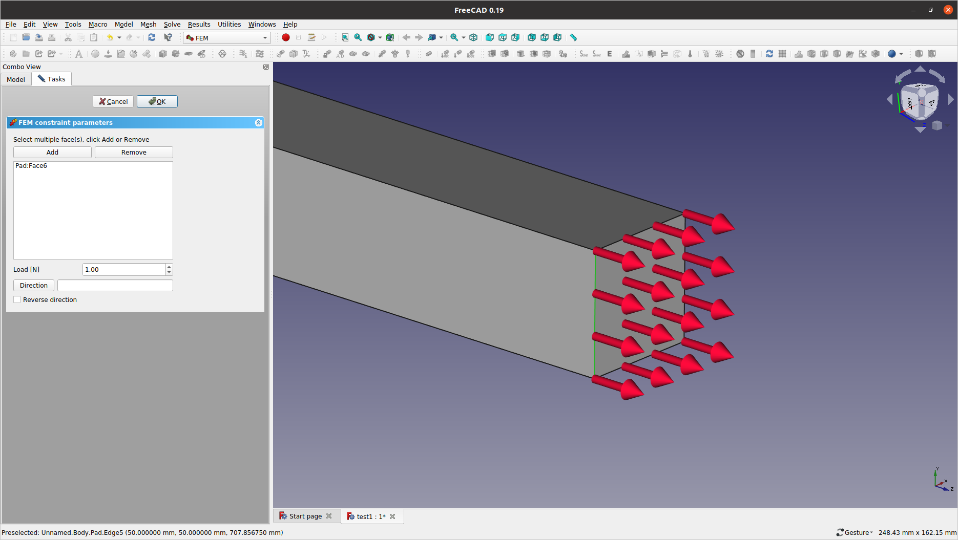
6.5: Then, click the Direction button in the Tasks pane (If in any case, the indicated direction is not what you wanted, you may tick on the Reverse direction option).
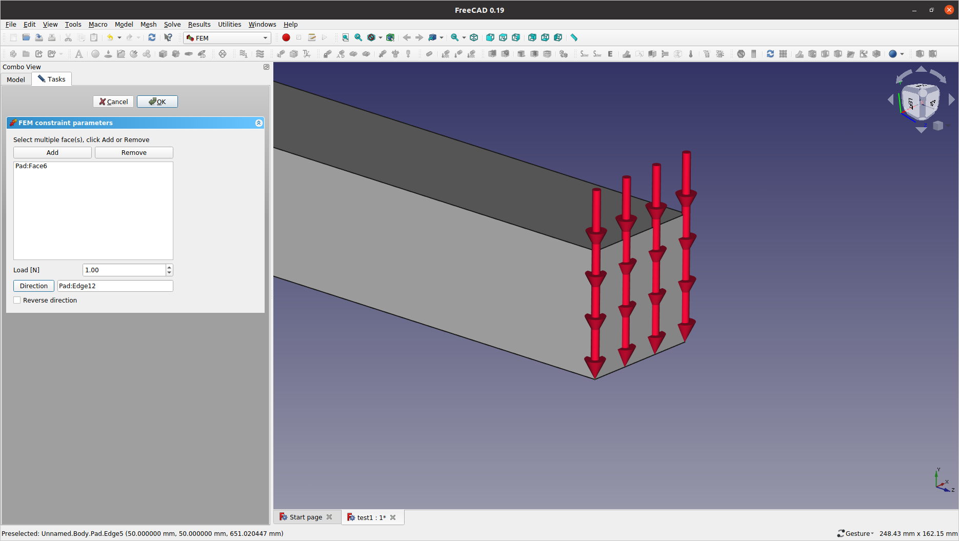
6.6: Now, enter the force value of 1000 for the Load [N] entry, and then confirm by clicking OK.

-
Ignore the
Links go out of the allow scopewarning from theReport viewpanel for now.
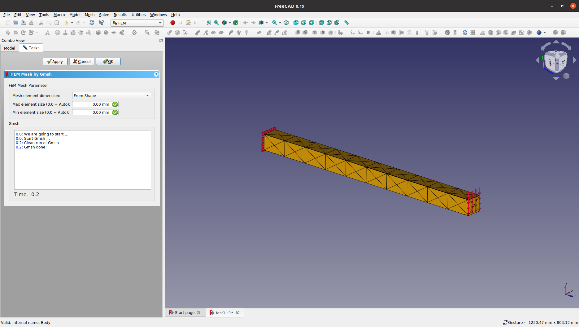
7: Mesh generation
To generate a FE mesh, you first need to pick the target object(s) to limit the meshing scope.
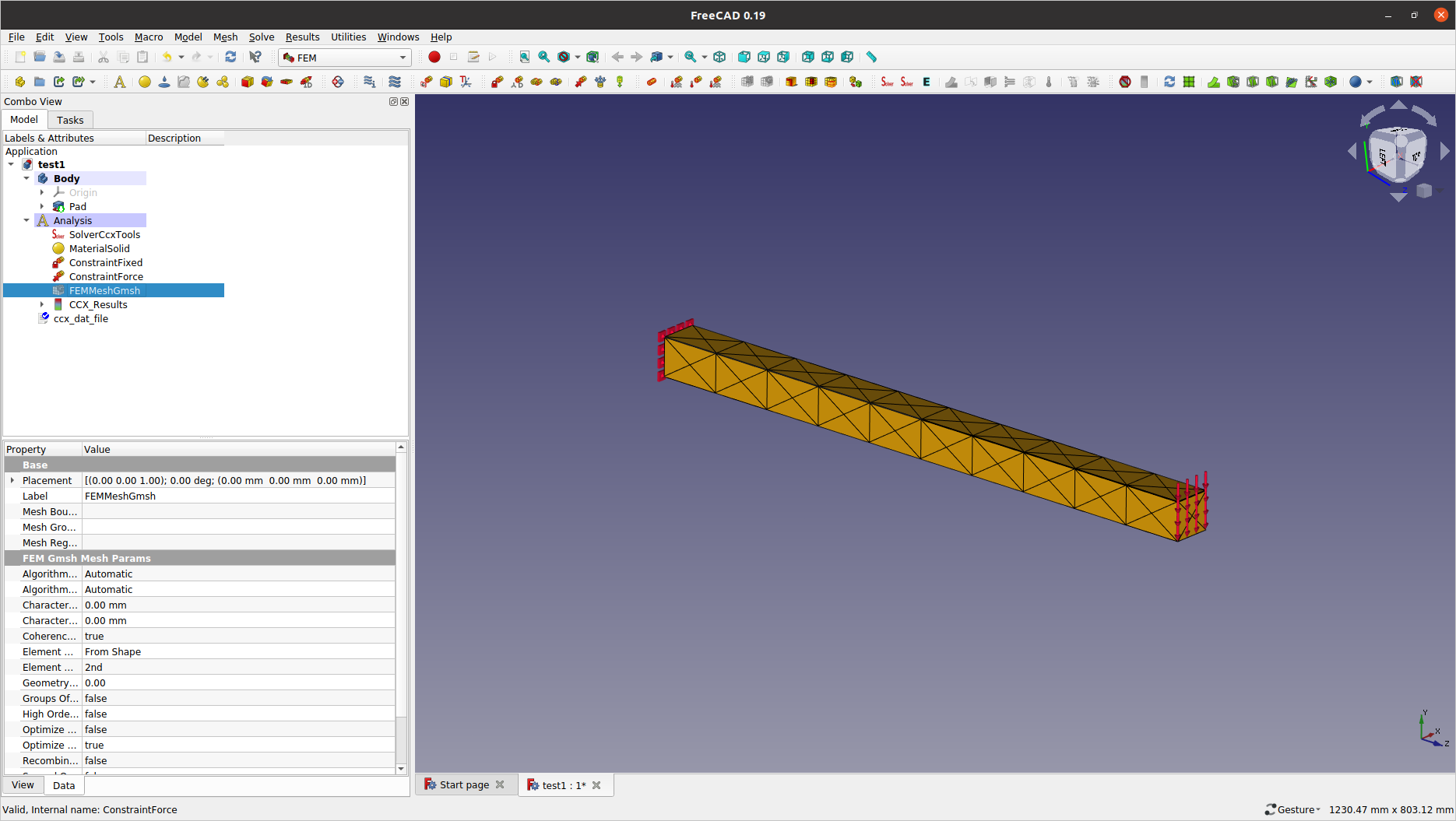
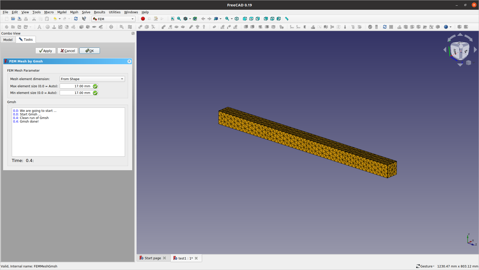
7.1: Select either the Pad object in the model tree — or the Body which is the same in this single-bodied example. Then, click the ![]() (
(Gmsh mesher) icon from the toolbar.
7.2: With the default setting accepted, click Apply to generate a pilot mesh; You may experiment with different sizing parameters later if time permits. Click OK for now.
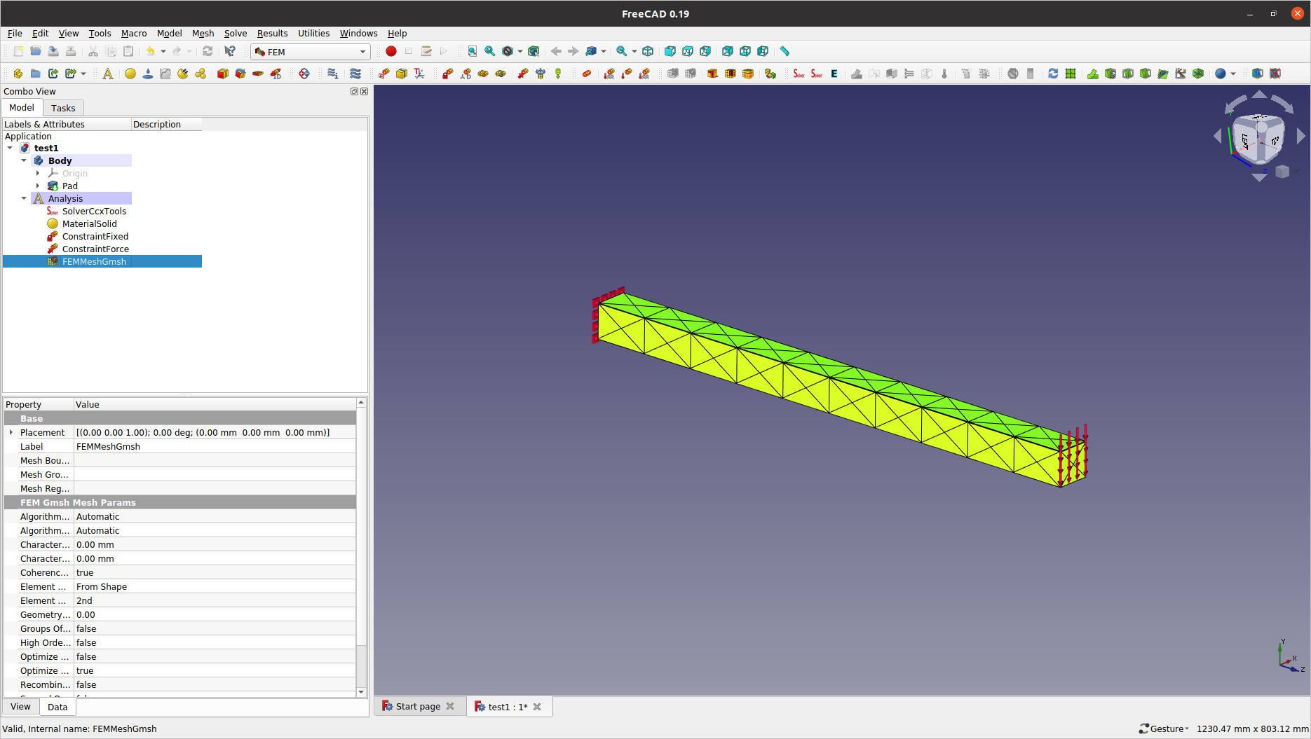
7.3 When you return from the mesher, the resulted mesh will be hidden. You can toggle the visibility of any visible objects by pressing the space bar with the target object selected in the model tree. Hide the mesh again before solving because the solver will reconstruct the mesh for the FE result (thus, two (2) mesh graphics in the display contexts will compete against each other).
8: Solving
Now with the geometry and FE mesh prepared, you can continue to solve the FE model.
8.1: Double-click the SolverCcxTools object in the model tree to open the Mechanical analysis panel. Check the Working directory (This is what you set from the FEM preferences in Step 4), and then click Write .inp file to initiate the solution data.

-
Make sure you click the
Write .inp fileeach time you redo the CalculiX computation — i.e. even if you have not started over the FEM Workbench.
8.2: At this point, you can check the auto-generated CCX input deck, by clicking the Edit .inp file button.
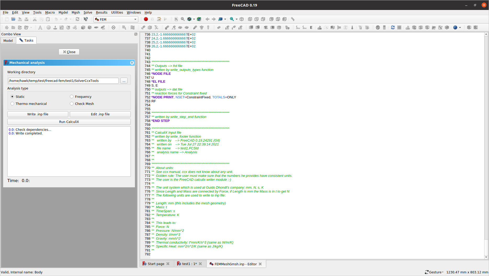
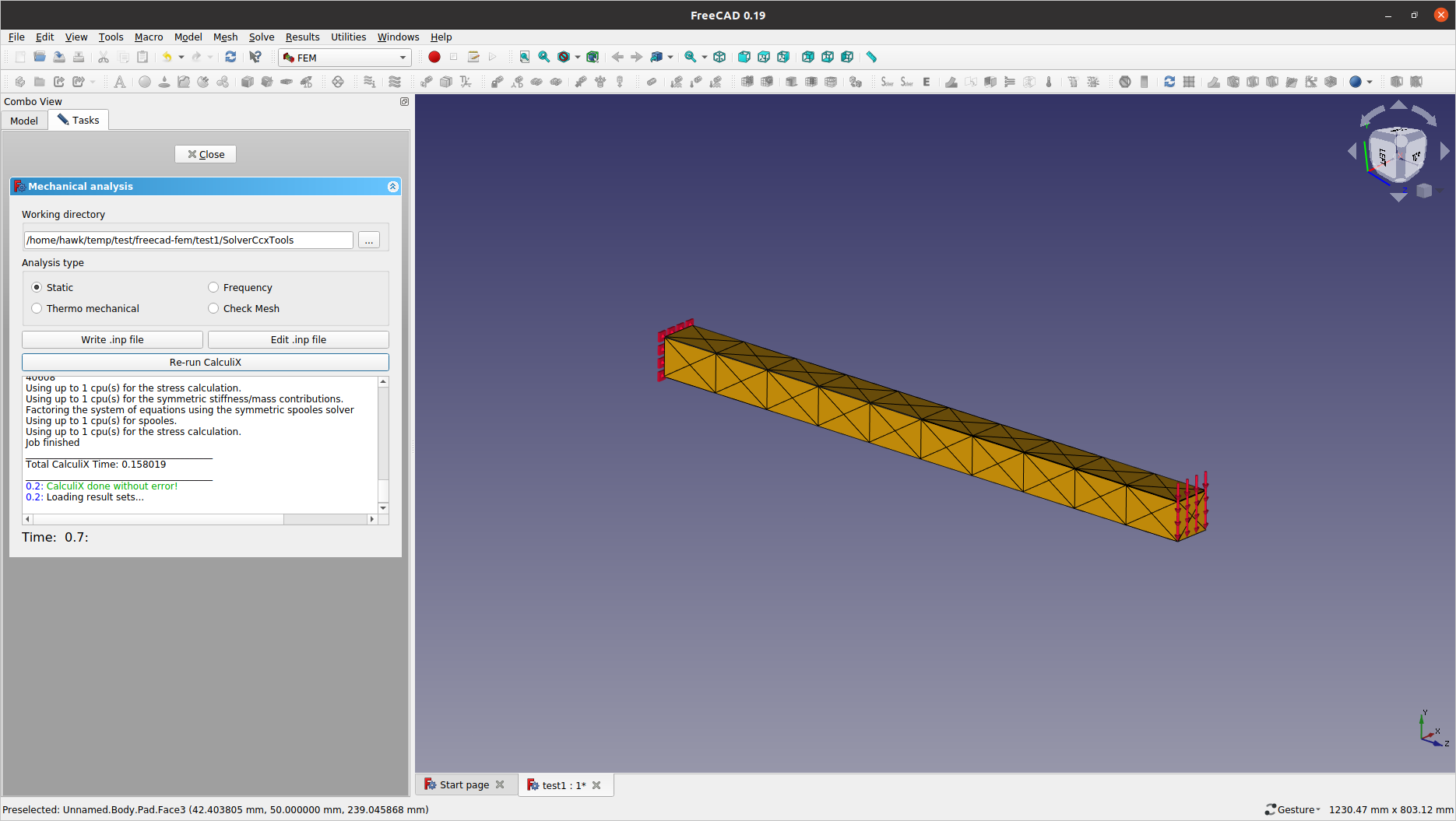
8.3: Close the input deck editor (if you opened it), and then click Run CalculiX. When done, click Close to exit from the Mechanical analysis panel.
-
Make sure that the
Mechanical analysispanel reported with the message,CalculiX done without error!.
9: Post-processing
9.1: Notice a new CCX_Results object is added to the Analysis branch. Double-click it to open the Show results panel.
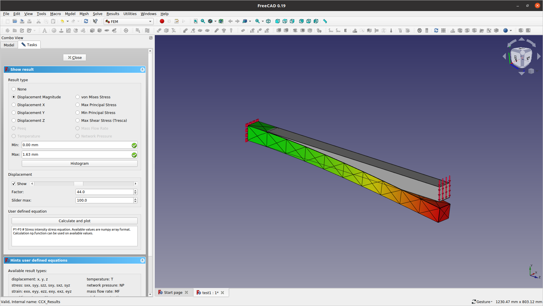
9.2: Select Displacement Magnitude for the Result type from the Show result panel.
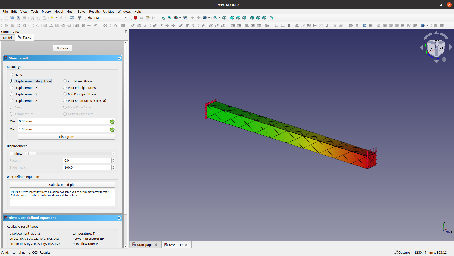
9.3: Also, tick on the Show in the Displacement section, and then move the scroll bar to the right to somehow exaggerate the displacement.
-
If wanting to hide the original shape from the graphics, visit the model tree — without closing the
Show resultpanel — to change the visibility for thePadobject. The same applies to the two (2) constraint graphics.
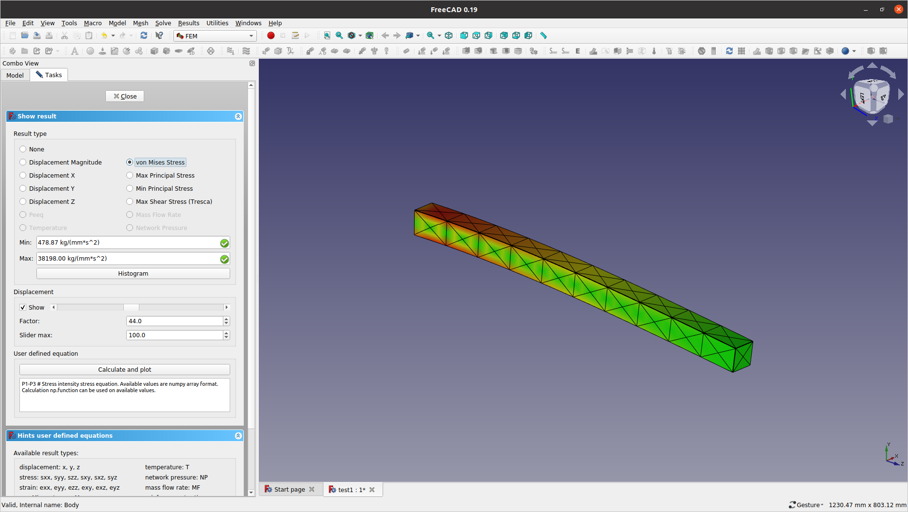
9.4: Investigate other FE result types such as von Mises Stress and Max Principal Stress.
10: (Optional) Results with a refined mesh
10.1: If time permits, try a finer mesh because the tetrahedral elements are known to be less accurate than the hexahedral ones, therefore require more (i.e. smaller) elements to match the hexahedral performance.
-
Remember that we turned off the visibility for the
Pad(and theFEMMeshGmsh) object(s). You can toggle their respective visibility from the model tree using the space bar.
10.2: With a refined element set, you have the option to define the "revised" case as a new document or to overwrite the whole database (treating the previous run as just a trial). In either case, make sure to click the Write .inp file button from the Mechanical analysis panel whenever re-running a new solver case. Note that, when you open the CCX_Results object after each re-run, the result will have been updated automatically.

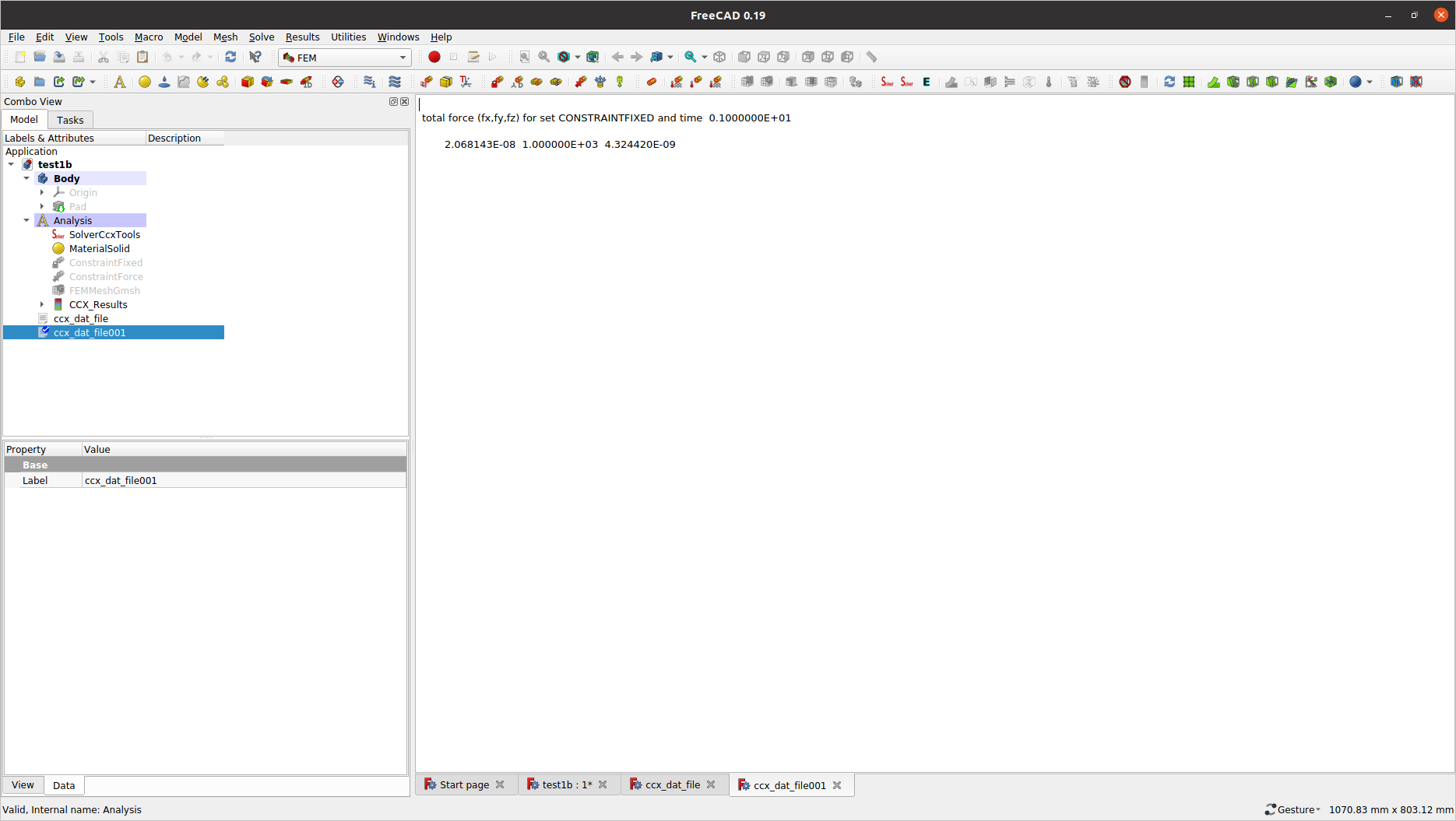
10.3: It is also worth noting that, the model tree remembers CalculiX text output (i.e. '.dat' data) for consecutive runs, which can serve as a quick parametric study with your FE model.